
Balanced spatial partitioning for point data in 20 lines
Published:
When working with geospatial data, sometimes a dataset is simply too large in its original form or file to be worked with effectively. I often work with hierarchical statistical models that function effectively when a larger dataset is partitioned into smaller subsets. To preprocess the data, I frequently need to find a way to split up a larger spatial domain into smaller pieces such that the number of objects or data points in each piece is roughly equal.
Unfortunately, I couldn’t find a quick reference online to do this with Python, so this post covers how to do it.
import geopandas         as gpd
import matplotlib.pyplot as plt

%config InlineBackend.figure_format = 'retina'
load_path ='../sample_data.gpkg'
gdf       = gpd.read_file(load_path).to_crs('epsg:2283')
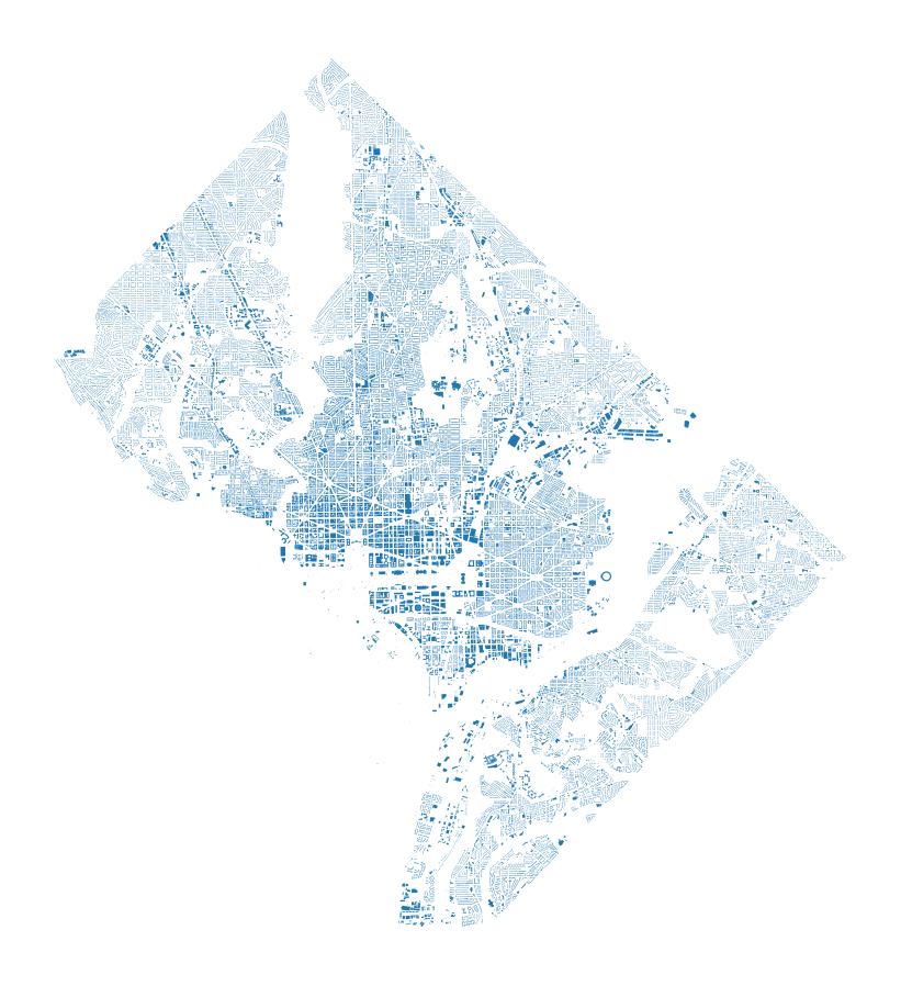
The data we’ll be working with is a set of building footprints for structures in Washington, DC. These have been collected from OpenStreetMap, and there’s roughly 134,000 of them:
print(len(gdf))
134846
As we can see from the plot below, these buildings aren’t already nicely spaced into even subsets. There’s many more in the urban core of Washington, DC. Also, the geometry of the region itself is somewhat irregular.
gdf.plot(figsize=(8,8)), plt.axis('off');
To split up the data, we’re going to use a recursive approach. The main data structure we’re working is going to be a list of tuples containing an x-coordinate, y-coordinate, and feature index, respectively. We will recursively split subsets of features into balanced north-south or east-west halves by bisecting a sorted array. If we denote the number of splits as $M$ and the number of features as $N$, this naive approach has a complexity of $\mathcal{O}(MN \log N)$ and thus scales well to large-ish datasets. We shouldn’t need to sort at each splitting, however, so really, this algorithm should be running in $\mathcal{O}(M+N \log N)$ time. I didn’t take the time to make that modification here since the original version was fast enough.
The top-level function (shown below) initializes the required variables and also post-processes the subsets by repeatedly flattening a nested list-of-lists until only the bottom-level results of the recursion are contained in a single top-level list.
def split(gdf, max_level):

    xs = (gdf.centroid.x.values, gdf.centroid.y.values, gdf.index.values)
    xs = list(zip(*xs))

    splits = split_recurse(xs, 0, max_level)

    for i in range(max_level-1):
        splits = sum(splits, start=[])

    indices_only = [[x[2] for x in subset] for subset in splits]

    return [gdf.loc[s] for s in indices_only]
The recursive function is defined below. It’s pretty simple - we just sort, split, and continue on with each subset. The parameter max_level controls how many partition cells there are; we do a binary split at each level, resulting in 2**max_level cells by the time we’re finished.
def split_recurse(xs, split_pos, max_level, level=1):

    xs.sort(key=lambda x:x[split_pos])
    mid = int(len(xs)/2)

    above = [pair for i, pair in enumerate(xs) if i > mid]
    below = [pair for i, pair in enumerate(xs) if i <= mid]

    subsets = [above, below]

    if level == max_level:
        return subsets
    else:
        # We flip between using the 0-th position and the 1st position in
        # our triplets to alternate between x- and y-coordinates for splitting.
        return [split_recurse(subset, 1-split_pos, max_level, level=level+1) for subset in subsets]
Let’s see how the results are distributed in space. The plot below shows the assignment of each building to a partition cell; each color is a different cell.
color_string = color='bgrcmykbgrcmykbgrcmykbgrcmyk'
plt.figure(figsize=(7,7))
gdf_splits = split(gdf, 5)

[subset.plot(ax=plt.gca(), color=color) for color, subset in zip(color_string, gdf_splits)];
plt.axis('off');

We can also see whether or not the subsets are balanced in size:
[len(subset) for subset in gdf_splits]
[4212,
 4214,
 4213,
 4215,
 ...
 4214,
 4215,
 4213,
 4215,
 4214,
 4215]
All of the cells have nearly the same number of points between them!