Modeling spatial structure in binary data with an H3 hexagonal coordinate system
Published:
We often model geostatistical (i.e. point-referenced data) in order to determine whether or not there are spatial patterns of autocorrelation. The object of interest is frequently an underlying spatial function giving rise to patterns of spatially correlated data. When we work with discrete observational data, a problem arises - we want to study smoothly-varying response surfaces over space, but the data themselves are not continuous and therefore we cannot specify a likelihood which is continuous in both space and response. Consequently, we often choose to reparameterize our model in terms of a latent smooth spatial surface and a link function mapping this spatial surface to the parameters of a likelihood function appropriate for discrete data.
This notebook shows how to analyze binary geospatial point data using a spatially-smoothing conditional autoregression model to test for the existence of clusters of 0 or 1 values. The dataset used in this example is simulated data of preterm births in Washington, DC. While many autoregressive models use square grids, we’re going to use a hexagonal tiling from Uber’s H3 coordinate system library to demarcate our areal units.
Generating simulated data
We begin by importing the requisite libraries and simulating synthetic data of preterm births.
import geopandas as gpd
import h3
import matplotlib.pyplot as plt
import networkx as nx
import numpy as np
import pandas as pd
import pymc3 as pm
import shapely

from sklearn.neighbors import BallTree

%matplotlib inline
%config InlineBackend.figure_format='retina'
To ensure reproducibility, it’s a good habit to include a version stamp as shown below.
%load_ext watermark
%watermark -iv
The watermark extension is already loaded. To reload it, use:
  %reload_ext watermark
h3        : 3.7.2
pymc3     : 3.11.1
shapely   : 1.7.1
geopandas : 0.8.1
numpy     : 1.18.5
pandas    : 1.1.3
matplotlib: 3.3.2
networkx  : 2.5
At several points we will need to use multiple functions to handle geospatial operations such as creating point data, determining the adjacency of vector features, and ensuring that sets of spatial objects are topologically connected. We’ll define them now so we can use them later.
def xy_from_gdf(gdf):
    '''
    Returns Nx2 matrix of X,Y coordinates from a GeoDataFrame
    '''
    return np.stack([gdf.centroid.x, gdf.centroid.y], axis=1)

def lat_lng_to_h3(point, h3_level):
    '''
    Applies H3's geocoding to determine the hexagonal cell
    containing a given point. The h3 level determines the
    size of the hexagonal lattice used.
    '''
    return h3.geo_to_h3(
      point.geometry.centroid.y, point.geometry.centroid.x, h3_level)

def add_geometry(row):
    '''
    Creates a vector feature from the H3 hexagonal coordinates.
    '''
    points = h3.h3_to_geo_boundary(
      row['h3'], True)
    return shapely.geometry.Polygon(points)

def nearest_neighbor_centroid(gdf1, gdf2, k=4):
    '''
    Vectorized operation for identifying the nearest points in gdf2 relative to gdf1.
    '''
    X_proposed, X_base = xy_from_gdf(gdf1), xy_from_gdf(gdf2)
    nearest = BallTree(X_proposed, leaf_size=2).query(X_base, k=k, return_distance=False)
    return nearest

def sigmoid(x):
    return np.exp(x) / (1 + np.exp(x))

def adjacency_via_buffer(gdf, very_small_distance=0.0003):
    '''
    Uses a spatial buffering and intersection operator to determine
    which features share a boundary in a GeoDataFrame.
    '''
    N = len(gdf)
    W = np.zeros([N,N], dtype=int)

    buffered = gdf.copy()
    buffered.geometry = buffered.buffer(very_small_distance)

    # Find neighbors by buffering and locating non-null overlap
    nearby  = buffered.geometry.apply(lambda x: np.where(buffered.intersection(x).area > 0)[0])
    nearest = nearest_neighbor_centroid(gdf, gdf, k=2)[:, 1:]

    for i, neighbors in enumerate(nearby):
        if len(neighbors) > 1:
            W[i, neighbors] += 1
            W[i,i]          -= 1 # self-neighboring is not allowed
        else:
            W[i, nearest[i]] = 1

    W = W+W.T > 0.
    W = W.astype(int)
    return W

def connect_components(W, geom_series):
    '''
    Iteratively add edges between nodes to the network
    until only a single edge-connected component covers the entire graph. This
    is critical for usage of the CAR model, which can fail if there
    are "islands" disconnected from each other in the network / adjacency matrix.
    '''
    connected = False
    while not connected:

        # Find the largest component and drop it from
        # the list of islands
        G = nx.convert_matrix.from_numpy_matrix(W)

        if nx.is_connected(G):
            break

        components = list(nx.connected_components(G))
        sizes      = [len(x) for x in components]
        largest    = np.argmax(sizes)
        components.pop(largest)

        # For each island, find the nearest node not on
        # the island and hook it up
        for island in components:
            element_on_island = list(island)[0]
            geom_on_island    = geom_series.iloc[[element_on_island]]
            repeated  = geom_on_island.iloc[np.zeros(geom_series.shape[0])]
            distances = geom_series.geometry.apply(lambda x: geom_on_island.distance(x))
            ordered_by_dist = np.argsort(distances.values[:,0])

            connected_for_island = False
            ctr = 0
            while not connected_for_island:
                proposed = ordered_by_dist[ctr]
                if proposed not in island:
                    W[element_on_island, proposed] = 1
                    W[proposed, element_on_island] = 1
                    print('Match for element {0} is {1}'.format(element_on_island, proposed))
                    connected_for_island = True
                ctr += 1

        G = nx.convert_matrix.from_numpy_matrix(W)
        connected = nx.is_connected(G)
    return W
Next, we use a shapefile of census tract data to determine how to sample birth events over space. We will use the population within each census tract, combined with a national average birth rate to determine how many births will be placed within each tract.
'''
Census tract shapefile taken from https://opendata.arcgis.com/datasets/f33d847161174e81ad59c9ea9c1f5a00_36.zip
'''
census_tract_path = "./data/Preliminary_2020_Census_Tract/Preliminary_2020_Census_Tract.shp"
tract_gdf = gpd.read_file(census_tract_path)
As we can see here, the POP10 field contains census counts.
tract_gdf.head()
| OBJECTID | STATEFP | COUNTYFP | TRACTCE | NAME | TRACTID | TRACTLABEL | POP10 | HOUSING10 | SHAPEAREA | SHAPELEN | geometry | |
|---|---|---|---|---|---|---|---|---|---|---|---|---|
| 0 | 21 | 11 | 001 | 001301 | 13.01 | 11001001301 | 13.01 | 3955 | 2156 | 2.882225e+06 | 8705.698378 | POLYGON ((-77.06943 38.95434, -77.06932 38.954... |
| 1 | 22 | 11 | 001 | 002001 | 20.01 | 11001002001 | 20.01 | 2340 | 1026 | 6.337953e+05 | 4198.601803 | POLYGON ((-77.04338 38.96146, -77.04329 38.961... |
| 2 | 23 | 11 | 001 | 003302 | 33.02 | 11001003302 | 33.02 | 2134 | 982 | 2.042153e+05 | 1915.794576 | POLYGON ((-77.01428 38.91506, -77.01275 38.915... |
| 3 | 24 | 11 | 001 | 008402 | 84.02 | 11001008402 | 84.02 | 2149 | 1270 | 2.741538e+05 | 2698.287213 | POLYGON ((-76.99497 38.89741, -76.99496 38.898... |
| 4 | 1 | 11 | 001 | 000101 | 1.01 | 11001000101 | 1.01 | 1384 | 999 | 1.993245e+05 | 2168.618432 | POLYGON ((-77.05714 38.91055, -77.05702 38.910... |
Our next step is to create a data table in which each row corresponds to a birth event and is associated with geospatial coordinates as well as a year.
base_pregnancy_rate = 11.4 / 1000 # births per thousand people
years = np.arange(2010, 2019)

birth_coords = []
birth_points = []

for year in years:

    for i, tract in tract_gdf.iterrows():
        tract_boundary = tract.geometry
        left, lower, right, upper = tract_boundary.bounds
        n_pregnancies = int(base_pregnancy_rate * tract['POP10'])

        for j in range(n_pregnancies):
            is_in_bounds = False

            while not is_in_bounds:
                coords = np.random.uniform(low=[left,lower],high=[right,upper])
                sample = shapely.geometry.Point(coords)
                is_in_bounds = tract.geometry.contains((sample))

            birth_points.append(sample)
            birth_coords.append(list(coords)+[year + np.random.uniform()])

birth_gdf = gpd.GeoDataFrame(data=birth_coords, columns=['lat','lon','year'], geometry=birth_points)
birth_gdf["year_int"] = birth_gdf['year'].astype(int)
birth_gdf.head()
| lat | lon | year | geometry | year_int | |
|---|---|---|---|---|---|
| 0 | -77.062823 | 38.951295 | 2010.816216 | POINT (-77.06282 38.95130) | 2010 |
| 1 | -77.056945 | 38.949016 | 2010.555112 | POINT (-77.05695 38.94902) | 2010 |
| 2 | -77.066707 | 38.951606 | 2010.082630 | POINT (-77.06671 38.95161) | 2010 |
| 3 | -77.062031 | 38.951623 | 2010.639241 | POINT (-77.06203 38.95162) | 2010 |
| 4 | -77.064879 | 38.955598 | 2010.950265 | POINT (-77.06488 38.95560) | 2010 |
To make this problem more interesting, we’ll simulate preterm births with spatial dependency. Our true generative process will allow for more preterm births in locations which are farther to the east and north.
birth_df   = pd.DataFrame(birth_gdf).drop(['geometry', 'year_int'], axis=1)
scales     = birth_df.std()
means      =  birth_df.mean()
zscore_gdf = (birth_df -means)/scales

# coefs are for lat, lon, and year respectively.
true_coefficients = [0.2, 0.2, 0.0]

# this value was chosen by hand to roughly line up with ~12% preterm births, on average
true_intercept    = -2
logits = zscore_gdf.dot(true_coefficients)+true_intercept

birth_gdf['preterm_prob'] = sigmoid(logits)

birth_gdf['preterm'] = np.random.binomial(1, birth_gdf['preterm_prob'])
birth_gdf['preterm'].mean()
0.12306756134464839
Let’s see the spatial point pattern for the births. The preterm births are marked in red while normal births are marked with blue points.
fig, axes = plt.subplots(2,2, figsize=(20,22), sharex=True, sharey=True)
axes = axes.ravel()

for i, year in enumerate(years[0:4]):
    birth_gdf.query(f"year_int=={year} & preterm==1").plot(markersize=5,
                                            color='red', ax=axes[i],zorder=1)

    birth_gdf.query(f"year_int=={year} & preterm==0").plot(markersize=2,
                                            color='blue', ax=axes[i],zorder=1, alpha=0.5)

    tract_gdf.plot(ax=axes[i], facecolor='none', edgecolor='k',zorder=2)
    preterm_frac = birth_gdf.query(f"year_int=={year}")['preterm'].mean()
    axes[i].set_title(f'Simulated births for {year}\n(Preterm fraction: {int(preterm_frac*100)}%)', fontsize=24)
    axes[i].axis('off')

plt.tight_layout()

A flaw of this simulation is that there are clearly jumps in point density at the interface between high- and low-population census tracts which are not reflective of reality.
Preprocessing spatial adjacency data
Since we don’t want to construct our model directly at the point level, we instead need to aggregate to a larger spatial unit. For this purpose, we’ll use the h3 library to aggregate into hexagonal bins.
h3_level = 9
gdf = birth_gdf
gdf['h3']      = gdf.apply(lat_lng_to_h3, h3_level=h3_level, axis=1)
gdf['hexagon'] = gdf.apply(add_geometry, axis=1)

hex_only = gdf[['hexagon','h3']].drop_duplicates(subset='h3')
hex_only = gpd.GeoDataFrame(geometry=hex_only['hexagon'], data=hex_only['h3'])
hex_only.sort_values(by='h3', inplace=True)

h3_to_int = {code: integer for integer, code in enumerate(np.sort(gdf['h3'].unique()))}
gdf['h3_int'] = gdf['h3'].apply(lambda x: h3_to_int[x])
print(hex_only.shape)
(1703, 2)
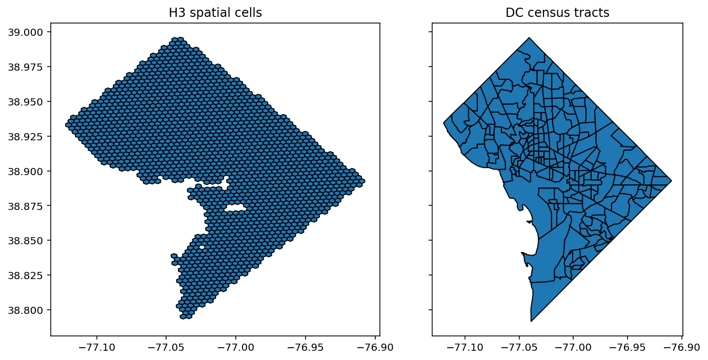
Under our model, each of the H3 cells is assumed to have its own free parameter for the probability of preterm birth. However, we will use the CAR prior to allow for pooling information across spatial cells and encouraging spatial smoothness in their estimates.
fig, axes = plt.subplots(1,2, figsize=(10,5), sharey=True)
hex_only.plot(ax=axes[0],edgecolor='k'), axes[0].set_title('H3 spatial cells')
tract_gdf.plot(ax=axes[1],edgecolor='k'), axes[1].set_title('DC census tracts')
plt.tight_layout()
As a final preprocessing step, we need to create the adjacency matrix $W$ and ensure that every node has a path through the adjacency matrix to every other path. Put more formally, we need to ensure there is only a single connected component in $W$ and that it is nontrivial.
# In geographic coordinate system
very_small_distance = 0.0003
W = adjacency_via_buffer(hex_only, very_small_distance=very_small_distance)
W = connect_components(W, hex_only)
To check the correctness of our procedures, we can make sure that every cell has at least neighbor and that no cell has more than six neighbors
neighbors_per_cell = W.sum(axis=0)

assert neighbors_per_cell.min() >= 1 & neighbors_per_cell.max() <= 6
Inference for model parameters
The probabilistic model we use has the following specification:
\[\alpha \sim Uniform(-0.95, 0.95)\\ c \sim Normal^{+}(0, 4)\\ \beta_0 \sim Normal(0, 9)\\ \mathbf{u}\sim CAR(W, \alpha)\\ y_j \sim Binomial(n_j, \sigma(u_j + \beta_0))\]Here, $Normal^{+}$ refers to the half-normal distribution with a mode at zero and almost all probability mass placed on the positive real line. Then, the CAR prior assumes that $\mathbf{u}$ has a multivariate normal distribution with a spatially-smoothed covariance matrix. The spatial smoothing is informed by the cellwise adjacency matrix $W$ and the spatial correlation parameter $\alpha$. Finally, the number of preterm births within the $i$-th spatial cell is assumed to follow a binomial distribution with its logit specified as the spatial effect plus an intercept.
preterm_counts = gdf.groupby('h3_int')['preterm'].sum()
total_counts   = gdf.groupby('h3_int')['preterm'].count()

n = len(preterm_counts)

with pm.Model() as model:
    # Hyperparameters on spatial correlation, random effect size, and model intercept
    alpha       = pm.Uniform('alpha',lower=-0.95, upper=0.95)
    scale       = pm.HalfNormal('scale', sd=2)
    intercept   = pm.Normal('intercept', sd=3)

    # Spatially-smoothing prior on logit of preterm birth probability
    spatial_effect = pm.CAR('spatial_effect', mu=0., W=W, alpha=alpha, tau=1., sparse=True, shape=n)
    likelihood  = pm.Binomial('likelihood', p=pm.math.sigmoid(spatial_effect*scale + intercept),
                             observed=preterm_counts.values, n=total_counts.values)

    # Applies Markov chain Monte Carlo to draw from the posterior distribution
    trace = pm.sample(target_accept=0.95, tune=2000)
<<!! BUG IN FGRAPH.REPLACE OR A LISTENER !!>> <class 'TypeError'> Cannot convert Type TensorType(float64, matrix) (of Variable Usmm{no_inplace}.0) into Type TensorType(float64, row). You can try to manually convert Usmm{no_inplace}.0 into a TensorType(float64, row). Elemwise{sub,no_inplace}(z, Elemwise{mul,no_inplace}(alpha subject to <function <lambda> at 0x7f5e61173c10>, SparseDot(x, y))) -> Usmm{no_inplace}(Elemwise{neg,no_inplace}(alpha), x, y, z)
Multiprocess sampling (4 chains in 4 jobs)
NUTS: [spatial_effect, intercept, scale, alpha]
Sampling 4 chains for 2_000 tune and 1_000 draw iterations (8_000 + 4_000 draws total) took 122 seconds.
The number of effective samples is smaller than 10% for some parameters.
Our posterior summary, as reported below, indicates strong evidence for spatial autocorrelation.
with model:
    print(pm.summary(trace, var_names=['scale', 'alpha', 'intercept']))
            mean     sd  hdi_3%  hdi_97%  mcse_mean  mcse_sd  ess_bulk  \
scale      0.483  0.036   0.411    0.547      0.001    0.001    1307.0
alpha      0.947  0.003   0.943    0.950      0.000    0.000    3294.0
intercept -1.983  0.026  -2.033   -1.936      0.001    0.001     363.0

           ess_tail  r_hat
scale        1876.0   1.00
alpha        1618.0   1.00
intercept     701.0   1.01
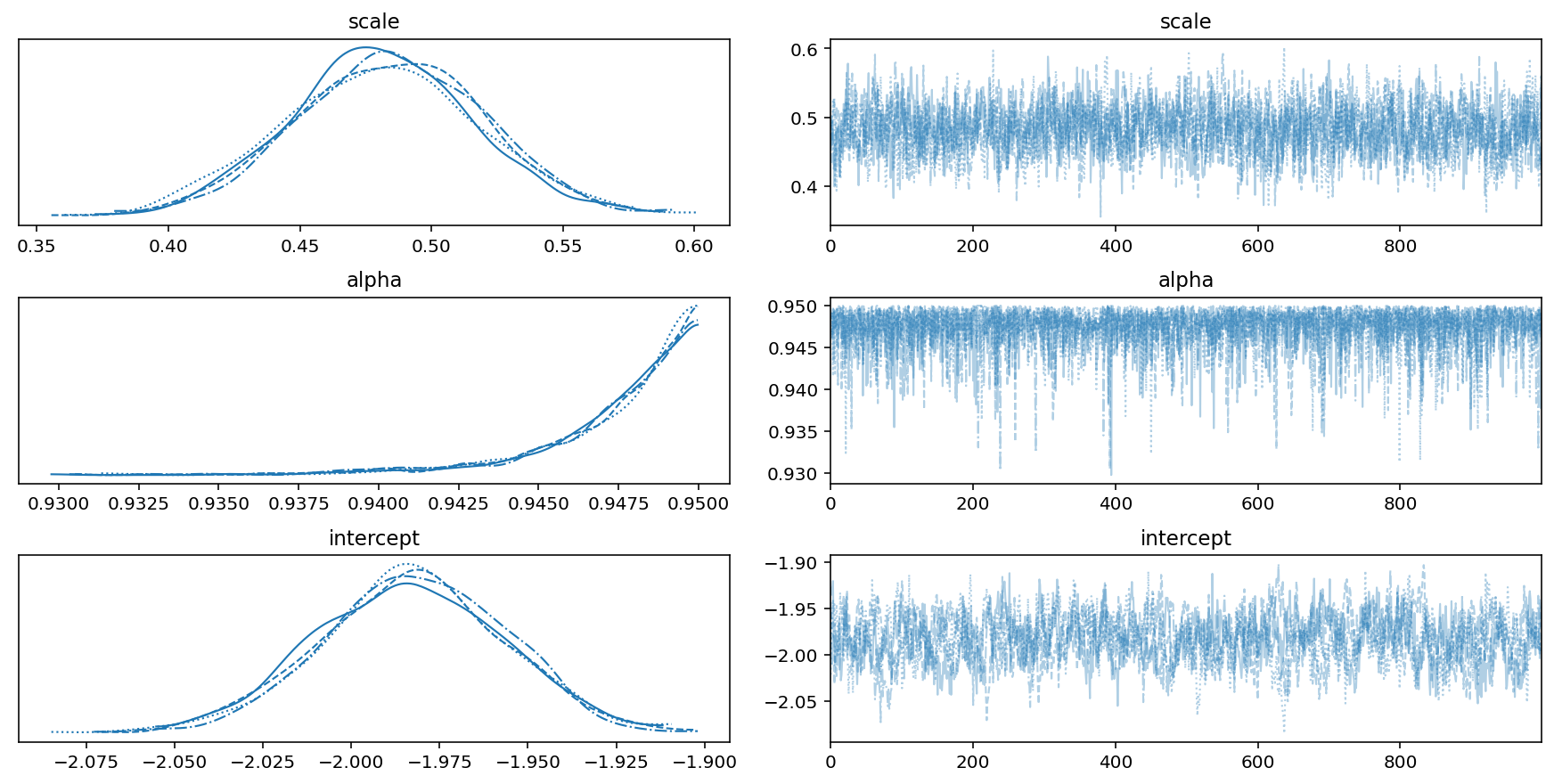
Our trace plots look good - no multimodality and the samples look uncorrelated. While the posterior for $\alpha$ is piling up near the edge of the boundary, this is fine.
with model:
    pm.plot_trace(trace, var_names=['scale', 'alpha', 'intercept'])
We next generate two plots to visualize the resulting estimates.
sigma_cutoff = 2

estimated_intercept = trace['intercept'].mean()

hex_only['preterm_fraction'] = (preterm_counts / total_counts).values
hex_only['estimate']   = trace['spatial_effect'].mean(axis=0)
hex_only['stdevs']     = np.abs(trace['spatial_effect'].mean(axis=0) / trace['spatial_effect'].std(axis=0))
hex_only['is_sig']     = hex_only['stdevs'] > sigma_cutoff
hex_only['delta_prob'] = sigmoid(hex_only['estimate']+estimated_intercept) - sigmoid(estimated_intercept)
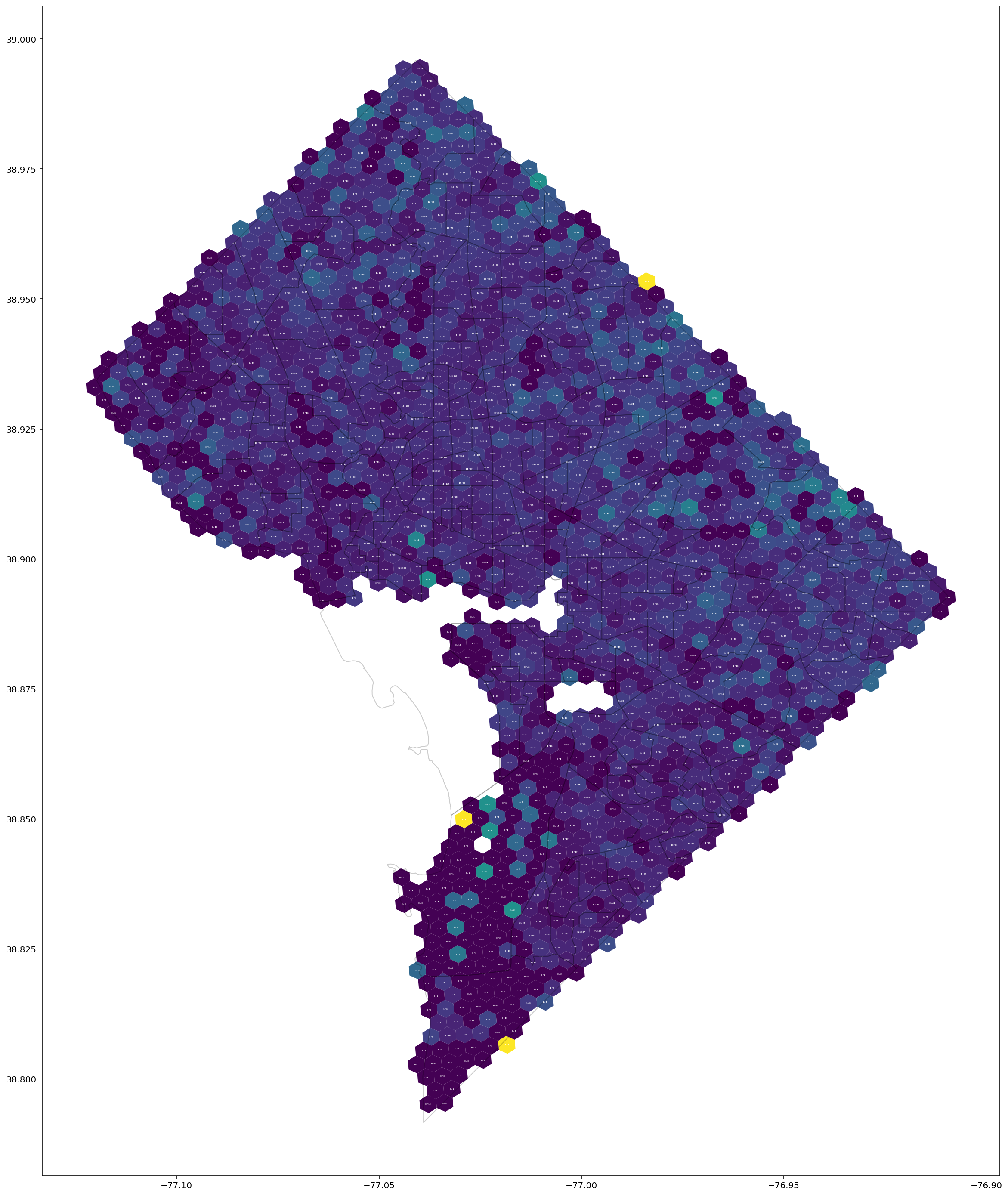
First, we create a plot of the data - the observed ratios of preterm births on a cell-by-cell basis.
fig, ax = plt.subplots(1, 1, figsize=(25,25))
hex_only.plot('preterm_fraction', ax=ax)
handle = tract_gdf.plot(facecolor='none', edgecolor='k',zorder=2,ax=ax, alpha=0.2, legend=True);

row_ctr = 0

for i, row in hex_only.iterrows():
    cent = row['geometry'].centroid
    ax.text(cent.x, cent.y,f'{preterm_counts.iloc[row_ctr]} / {total_counts.iloc[row_ctr]}',
                 ha='center', va='center',fontsize=2, fontweight='bold', color='w')
    row_ctr += 1
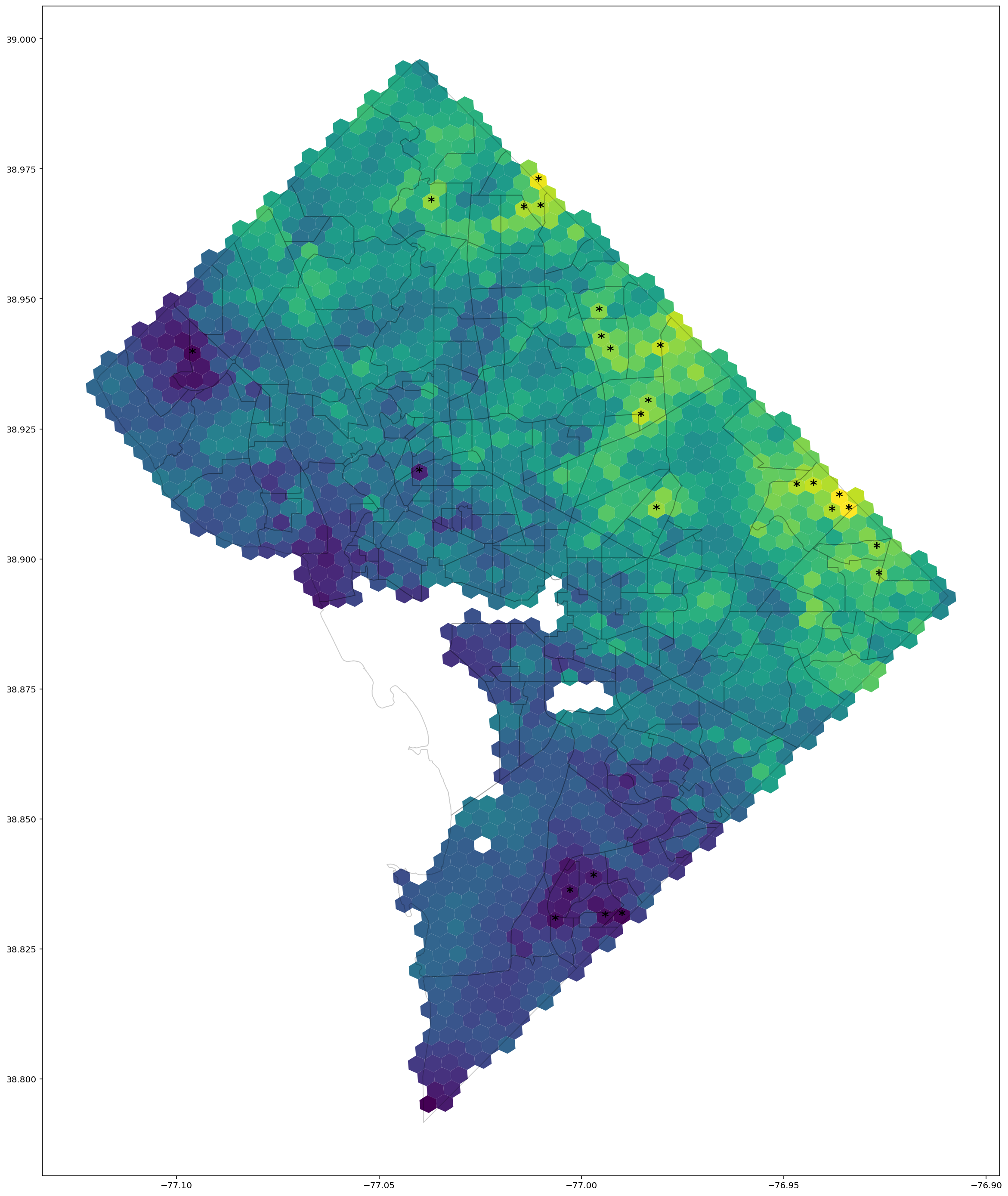
Next, we compare against our inferred estimates. Cells for which our estimate of the spatial effect is significant at the $2\sigma$ level are highlighted with a star.
ax = hex_only.plot('estimate',figsize=(25,25))
tract_gdf.plot(facecolor='none', edgecolor='k',zorder=2,ax=ax, alpha=0.2, legend=True)

for i, row in hex_only.iterrows():
    cent = row['geometry'].centroid
    if row['is_sig']:
        sig_str = '*'
    else:
        sig_str = ''
    se = row['delta_prob']
    ax.text(cent.x, cent.y, sig_str, ha='center', va='center',fontsize=16, fontweight='bold')

axes[0].set_title('Simulated preterm birth ratio', fontsize=24)
axes[1].set_title('Inferred change in probability of preterm birth', fontsize=24);