A recurring theme in my posts is the power of combined statistical and physical/mechanistic models that are really only possible with modern Markov Chain Monte Carlo (MCMC) frameworks. In this post, I’ll go over how to make a statistical model out of a simple dynamical system. Let’s assume we have a system governed by the following equations: \(\frac{dx}{dt} = -a\cdot x(t) + y(t)\) where \(y\) is a forcing variable that varies over time. Both \(x\) and \(y\) are observed but \(a\) is unknown. We want to make a statistical inference about the values of \(a\) and we’ll employ PyMC3 to do this.
As is the case in many of my other posts, we’ll be using a combination of Theano and PyMC3 for the model composition and inference. Numpy and Matplotlib are used to help generate dummy data and visualizations. In previous versions of PyMC and other frameworks such as Stan, we’d build in the dynamic feedback structure of \(x\)’s differential equation by using a for loop or a similar construct. Because Theano build a computational graph as opposed to immediately evaluating statements, we can’t do this and will have to use the scan function from Theano instead.
import theano.tensor as tt
import pymc3 as pm
import numpy as np
import theano
import matplotlib.pyplot as plt
%matplotlib inline
Most of the code below is pretty self-explanatory. We are going to create a 1D Numpy array with \(T\) elements and drive it according to the dynamics of the equation I wrote above. Then, we’ll add some noise to it.
T = 100 # Number of timesteps
# Generate random noise
noise_stdev = 0.1
noise = np.random.randn(T) * noise_stdev
# We create a relatively sparse external forcing series
y = np.random.randn(T)
y[y > -1.5] = 0
a = 0.1 # Model's lone parameter
x0 = 1 # Initial value
# This function does a simple forward integration of the ODE
def f(x0,y,noise,a,T):
x = np.zeros(T)
x[0] = x0
for i in range(1,T):
x[i]=x[i-1] - a*x[i-1]+y[i]
return x+noise
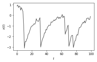
# Generate and plot the data
data = f(x0,y,noise,a,T)
plt.figure(figsize = (5,3))
_ = plt.plot(data,color = '0.3'),plt.ylabel('$x(t)$'),plt.xlabel('$t$')
This is essentially a system which is continually trying to return back to the origin and oscillate about zero but it is driven by occasional shocks \(y(t)\) which are independent of the values of \(x(t)\)
The structure of this model borrows heavily from the PyMC3 tips and heuristics page. It’s a great resource for building nontrivial Bayesian models. Also, the PyMC3 Discourse site is an invaluable resource.
This is where things get a little tricky. To summarize, we are going to create a function fn_step that does the forward integration similarly to the function I made in the previous code cell except it does it for just a single timestep using 1) the current timestep’s forcing value \(y(t)\), the previous timestep’s state value \(x(t-1)\) and the model parameter \(a\). We are declaring this because the Theano scan function needs fn_step (or a lambda function) as an argument to contruct its own pseudo-for loop in the Theano computational graph.
# The order of the arguments is very important - it must be exactly this way.
# see the Theano scan documentation for the reason why.
def fn_step(current_y,previous_x,coeff):
    # Even though this looks like just a normal Python function,
    # because it is using standard Python operators and Python is
    # not a strongly typed language, Theano can use this
    # and just drop in its own operators to overload + and *.
    return previous_x - coeff*previous_x + current_y
For any function that we pass to scan, the arguments have to be in this order: first, the values of any external sequences, i.e. anything that is not going to be modified or altered by scan. In this case, it’s the driving variable \(y(t)\) which is external to the system. Followed by that comes the value of the looped-over quantity at a previous timestep. If more than one timestep needs to be passed to the function then a more elaborate construction is needed and the theano literature refers to the timesteps as ‘taps’. Finally, any non-sequence values are passed to fn_step. Here, we have only a single one of these which is our model parameter \(a\). If there are multiple external sequences, multiple output series or multiple non-sequence values, then this general structure still holds but there are additional considerations. Just read the help text for scan.
Now that we have the system equation written out (and with syntax that Theano can work with later, so no Numpy or other non-Theano functions), we need to set up a distribution that makes the system model probabilistic.
from pymc3.distributions import distribution
floatX='float32' # This is just to fix an annoying casting issue that comes up when using scan

class Dynamical(distribution.Continuous):

    def __init__(self,coeff,sd,x0,y,*args,**kwargs):
        super(Dynamical,self).__init__(*args,**kwargs)
        self.coeff = tt.as_tensor_variable(coeff)
        self.sd    = tt.as_tensor_variable(sd)
        self.x0    = tt.as_tensor_variable(x0)
        self.y     = tt.as_tensor_variable(y)

    # The uses of tt.cast are just to fix casting mismatches between float32 and float64 variables
    def get_mu(self,x,x0,coeff,y):
        # Here, we are saying that the vector mu is calculated by iteratively applying
        # the forward equation 'fn_step' and that it uses external sequence 'y'
        # along with initial value 'coeff' (i.e. a scalar and non-sequence variable).
        # The info about the output is the initial value 'x0'.
        mu,_ = theano.scan(fn = fn_step, outputs_info = tt.cast(x0,floatX),
                     non_sequences=tt.cast(coeff,floatX),
                           sequences=tt.cast(y,floatX))
        return mu

    def logp(self,x):
        mu = self.get_mu(x,self.x0,self.coeff,self.y)
        sd = self.sd
        return tt.sum(pm.Normal.dist(mu = mu,sd = sd).logp(x))
Let’s break this down: the class Dynamical is going to be used like any other PyMC3 distribution; we will pass its constructor the usual distribution init arguments such as a name, shape and parameters. However, the likelihood function for this distribution is going to reflect how close the observed values of \(x\) are to the simulated values using Monte Carlo samples of the model parameter \(a\). For more examples, I recommend several other pages. First, look at the documentation for scan on the Theano webpage and also check out its help text which is invaluable in sorting out the order and purpose of the arguments. Next, look at the PyMC3 time series distribution code to see how they’ve used it for a vector autoregression with \(p\) lags. Finally, you can follow the template for a conditional autoregression model on the PyMC3 website. The sd parameter just controls how much we penalize the simulated value of \(x\) given a sample of \(a\) relative to the observed value of \(x\) that we have.
with pm.Model() as model:
    a_parameter = pm.Normal('a_parameter')
    sd = pm.HalfNormal('sd',sd = 0.2)
    x0 = pm.Flat('x0')
    x_testval = np.ones(len(y),dtype=np.float64)
    x  = Dynamical('x',coeff = a_parameter, sd= sd, x0=x0, y = y,shape = len(y),
                   testval=x_testval)

    observations = pm.Normal('observations',mu = x, sd = 0.01,observed=data)
    trace = pm.sample() # Automatically applies the built-in No-U-Turn sampler
100%|██████████| 1000/1000 [00:24<00:00, 41.17it/s]
You can see that once we have the Dynamical distribution set up, the rest of the model is straightforward. I have put a prior on the noise variance to prefer lower values (though still confined to be a positive, real number with HalfNormal) and a flat prior on the initial value of x0. I have also set x_testval as the PyMC3 model won’t know what value of \(x\) to start with as I did not give Dynamical a method to automatically set an initial value. You can see that the sampler is fairly slow for this example - the No-U-Turn sampler is essentially navigating the parameter space with backpropagation through 300 \(T\) timesteps as I have not truncated the gradient calculations. Still, it finishes in a reasonable amount of time for this simple case.
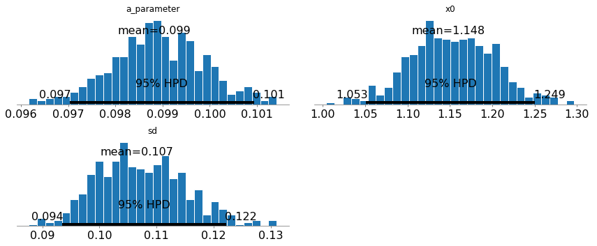
Below, the posterior plots show that we recover the value of \(a\) and \(x(0)\) with a very high precision. We also see that the noise standard deviation is properly recovered too.
_ = pm.plot_posterior(trace,varnames=['a_parameter','x0','sd'])
In later posts I’ll extend this to create Bayesian versions of some simple hydrology models. We’ll follow the same recipe but with substantially more complexity in the function fn_step.