Easy local average with Google Earth Engine’s Python API

Across many projects, I’ve needed to analyze remote sensing data and compute, for some points or polygons, a statistical summary of the remotely sensed layer in a neighborhood of those objects. Sometimes, that summary needs to be exactly calculated within the extent of the spatial object (like the boundaries of a field or a county) but other times, simply knowing the average in a circular or square buffer around the feature is good enough.

I wrote this notebook to show what is the least painful way to do it for large numbers of geometries without having to manually retrieve and download data. We do this by making use of the functionality in Google’s Earth Engine via its Python API. In this example, I calculate the average amount of surface water within a 1 km. circular buffer around 100,000 points sampled within the vicinity of Washington, DC.

The imports we require are fairly standard. I’ve used contextily here only to show a basemap comparison later on - you can omit this with no ill effect. Otherwise, we use the ee library for Earth Engine as well as Geopandas and the built-in json library.

import contextily as ctx
import ee
import geopandas  as gpd
import json
import numpy      as np

from shapely   import geometry
from time      import time

The first thing we’ll do is create some fake data. Here, I randomly sample a large number of points as referenced by their latitude / longitude coordinates within a bounding box.

left, lower, right, upper=-77.14,38.81,-76.90,38.99

n     = 100_000
longs = np.random.uniform(left, right, size=n)
lats  = np.random.uniform(lower, upper, size=n)

gdf        = gpd.GeoDataFrame(geometry=[geometry.Point(x,y) for x,y in zip(longs,lats)], 
                crs='epsg:4326')
n_geoms    = len(gdf)

Next, we’ll indicate that the remote sensing image we want to average over is the Global Surface Water binary yes/no water layer which indicates, for each pixel, whether or not water was ever sensed in that pixel over the entire Landsat archive. We also define how big we want our local summary buffer to be, in terms of meters.

image         = ee.Image("JRC/GSW1_3/GlobalSurfaceWater").select("max_extent")
radius_meters = 1000

The most important part of this is the next code block. After instantiating an EarthEngine FeatureCollection corresponding to our points, we convolve the target image with a circular kernel around the points that we’ve supplied. We then ask Earth Engine to directly evaluate these summaries and then put them into our local memory.

def radial_average(ee_geoms, image, radius_meters):
    '''
    Creates EE object for zonal average about each
    point in <ee_geoms> and directly evaluates it
    into the local kernel.
    '''

    kernel = ee.Kernel.circle(radius=radius_meters,
                              units='meters',
                              normalize=True);

    smooth = image.convolve(kernel);

    val_list = smooth.reduceRegions(**{
        'collection':ee_geoms,
        'reducer':ee.Reducer.mean()
    }).aggregate_array('mean')

    val_array = ee.Array(val_list).toFloat().getInfo()
    return val_array

This loop takes our GeoDataFrame of points from earlier and splits it into smaller blocks so that we don’t hit the Earth Engine data transfer limit. We use the JSON representation of our GeoDataFrame to make it palatable to Earth Engine.

block_size    = 10000
n_requests    = int(n_geoms/block_size)

blocks = np.array_split(gdf, n_requests)

vals  = []
start = time()

ee.Initialize()

for gdf_partial in blocks:
    js           = json.loads(gdf_partial.to_json())
    ee_geoms     = ee.FeatureCollection(js)
    partial_vals = radial_average(ee_geoms, image, radius_meters)
    
    vals += [partial_vals]
    print(time() - start)
    start = time()
    
vals = np.concatenate(vals)

8.036774396896362
7.84600043296814
7.808760643005371
6.694471120834351
8.156326532363892
7.155316114425659
7.938997268676758
6.8641228675842285
6.573741436004639
7.0107102394104

Overall, it takes about 80 seconds for this to run. It could certainly be done faster locally with GDAL and/or zonalstats, but that requires extra setup and storing the data locally.

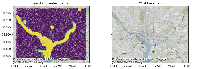
To verify that our results are sensible, we overlay our point summaries with an OpenStreetMap-derived basemap for Washington DC.

fig, axes = plt.subplots(1,2,figsize=(11,5), sharey=True)
axes[0].scatter(longs,lats, c=vals, vmax=0.05, s=0.05)
axes[1].scatter(longs,lats, alpha=0.001)
[ctx.add_basemap(ax, crs='epsg:4326') for ax in axes]

axes[0].set_title('Proximity to water, per point')
axes[1].set_title('OSM basemap')

plt.tight_layout();