Density estimation for geospatial imagery using autoregressive neural models
Published:
Bayesian machine learning is all about learning a good representation of very complicated datasets, leveraging cleverly structured models and effective parameter estimation techniques to create a high-dimensional probability distribution approximating the observed data. A key advantage of posing computer vision research under the umbrella of Bayesian inference is that some tasks become really straightforward with the right choice of model.
In this notebook, I show how to use PixelCNN, a deep generative model of structured data, to perform density estimation on geospatial topographic imagery derived from LiDAR maps of the Earth’s surface. I also highlight how easy this is within TensorFlow Probability, a new open-source project extending the capabilities of Tensorflow into probabilistic programming, i.e. the representation of probability distributions with computer programs in a way that treats random variables as first-class citizens.
Note: To reproduce this notebook, you will need the digital elevation map dataset I used to train the model. It’s too large to be hosted on my Github repository. Email me at ckrapu at gmail.com to get everything you need to reproduce this!
Density estimation
Density estimation is a task which has a common sense interpretation: if our understanding of the world is encoded in a probabilistic model, data points with especially low density are rare according to the model while points with high density are common. Suppose that you are walking down the street and you see a bright, neon blue dog that is as large as a firetruck. This is an instance which would probably receive low density under your subjective model of the world because there is exceedingly low probability of it appearing. Conversely, a smaller brown dog would receive a higher density value because it is more likely under the set of beliefs and assumptions you hold about the world.
Most probability distributions are not as rich or flexible as the set of beliefs that we individually hold about the world. Coming up with extremely flexible and rich distributions is an active area of research. As of right now, a leading approach to generating these distributions is via neural autoregressive models which extend standard time series models such as the autoregressive or ARIMA models to have a neural transition operation rather than a linear, Markovian operation. The PixelCNN architecture is a popular neural autoregressive model currently in use.
Many machine learning models of imagery do not allow for easy density estimation. For example, the variational autoencoder provides a mapping from latent variable $\mathbf{z}$ to observed data point $\mathbf{x}$. Unfortunately, calculating $p(\mathbf{x})$ under the model typically requires approximating the integral $p(\mathbf{x}) = \int_z p(\mathbf{x}\vert \mathbf{z})p(\mathbf{z}) d\mathbf{z}$. Autoregressive models, in their most basic form, just don’t have this latent variable representative and instead parameterize the function $p(x_i \vert x_{i-1},…,x_1)$ where $x_i$ denotes the $i$-th pixel in the image. This admits a decomposition of the image’s probability as $p(\mathbf{x})=\prod_i p(x_i\vert x_{i-1},…,x_1)$. This assumes a total ordering of the pixels in an image; we usually assume the raster scan order (though there are creative solutions which can improve on this!).
The rest of this post shows how to use the PixelCNN distribution from Tensorflow Probability and apply density estimation. The PixelCNN distribution was included with the 0.9 update of tensorflow-probability, so you’ll need to upgrade your installation if you were on 0.8 or earlier.
import tensorflow as tf
import tensorflow_probability as tfp
import numpy as np
import matplotlib.pyplot as plt


from utils import flatten_image_batch
print(f'This script uses Tensorflow {tf.__version__}')
print(f'Tensorflow Probability version: {tfp.__version__}')
This script uses Tensorflow 2.1.0
Tensorflow Probability version: 0.9.0
The dataset that I’m using consists of images with dimension $32\times32\times1$ representing topographical maps of the Earth’s surface in the state of North Dakota. Each pixel’s single channel of data represents the average elevation across several square meters. Features like roads, ditches, rivers and valleys can be seen in these images.
data_numpy = np.load('../data/datasets/training/dem_32_filtered.npy').astype('float32')
dem_as_int = (((data_numpy + 1)/2) * 255).astype(np.uint8)
Currently, the available architectures for PixelCNN work best when the output data is quantized. The image data originally had pixel values within the rage $[-1,1]$ which need to be mapped to ${0,1,…,255}$. Let’s take a look below and see what these images look like:
selected = np.random.choice(np.arange(data_numpy.shape[0]),size=36,replace=False)
images = dem_as_int[selected][0:32]
flat = flatten_image_batch(images.squeeze(),4,8)
plt.figure(figsize=(16,8))
plt.imshow(flat), plt.title('Training data'),plt.gca().axis('off');
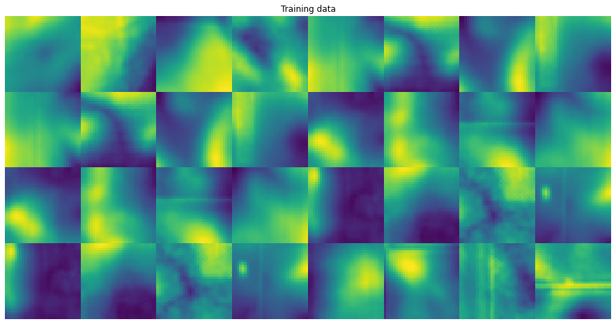
Many of the images are of gently sloped or rolling surfaces with a few linear features such as ditches or roads. Many of the images have local regions of high variance corresponding to marshy vegetation which scatters the LiDAR pulses used for elevation estimation.
The PixelCNN model is actually a joint distribution over all the pixels of an image. Thus, it was possible for the developers of the tensorflow-probability package to actually include it as one of their distributions! This makes it really easy to work with and the code below shows how little setup is required to train a PixelCNN with TFP. Much of this code was copied from the TFP documentation.
# Specify inputs and training settings
input_shape = (32, 32, 1)
batch_size = 16
epochs = 3
filters = 96

# Create a Tensorflow Dataset object
train_dataset = tf.data.Dataset.from_tensor_slices(dem_as_int)
train_it = train_dataset.batch(batch_size).shuffle(data_numpy.shape[0])

# Create the PixelCNN using TFP
dist = tfp.distributions.PixelCNN(
    image_shape=input_shape,
    num_resnet=1,
    num_hierarchies=2,
    num_filters=filters,
    num_logistic_mix=5,
    dropout_p=.3,
)

# Define the model input and objective function
image_input = tf.keras.layers.Input(shape=input_shape)
log_prob = dist.log_prob(image_input)

# Specify model inputs and loss function
model = tf.keras.Model(inputs=image_input, outputs=log_prob)
model.add_loss(-tf.reduce_mean(log_prob))
Once the model is specified, we just need to compile it and start training. PixelCNN is an example of an autoregressive model and these are notorious for taking a long time to train. Unfortunately, I only have access to a single GPU currently. Normally, this code would display a progress bar and training metrics. I’ve toggled these off to keep the document short and prevent a large number of warnings from being shown.
# Compile and train the model
model.compile(
    optimizer=tf.keras.optimizers.Adam(.001),
    metrics=[])

history = model.fit(train_it, epochs=epochs, verbose=True)
WARNING:tensorflow:Output tf_op_layer_Reshape_3 missing from loss dictionary. We assume this was done on purpose. The fit and evaluate APIs will not be expecting any data to be passed to tf_op_layer_Reshape_3.
Train for 4602 steps
Epoch 1/3
3626/4602 [======================>.......] - ETA: 30:48 - loss: 2357.9549

IOPub message rate exceeded.
The notebook server will temporarily stop sending output
to the client in order to avoid crashing it.
To change this limit, set the config variable
`--NotebookApp.iopub_msg_rate_limit`.

Current values:
NotebookApp.iopub_msg_rate_limit=1000.0 (msgs/sec)
NotebookApp.rate_limit_window=3.0 (secs)


4602/4602 [==============================] - 8735s 2s/step - loss: 1989.1206
Epoch 3/3
 612/4602 [==>...........................] - ETA: 2:06:25 - loss: 1972.0003
Since we’ve created an approximation of a probability distribution, we can sample from it to see examples of points that have high density under the PixelCNN model. As a warning, this sampling procedure can take quite awhile.
samples = dist.sample(36)
Let’s visually compare the sampled values with ground truth data points.
from utils import flatten_image_batch

samples_numpy = samples.numpy().squeeze()
flat_samples = flatten_image_batch(samples_numpy,6,6)
plt.figure(figsize=(6,6)),plt.imshow(flat_samples),plt.title('Simulated images')
plt.gca().axis('off')

selected = np.random.choice(np.arange(data_numpy.shape[0]),size=36,replace=False)
flat_ground_truth = flatten_image_batch(data_numpy[selected].squeeze(),6,6)
plt.figure(figsize=(6,6)),plt.imshow(flat_ground_truth),plt.title('True images')
plt.gca().axis('off');
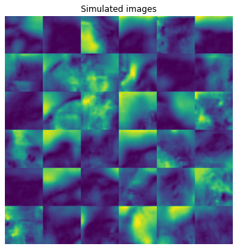
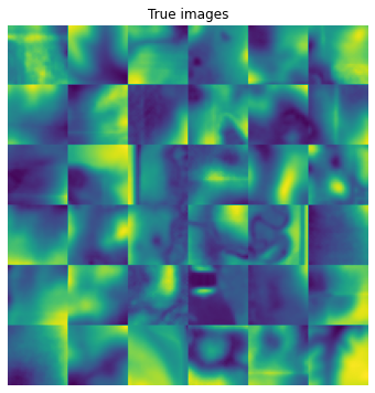
Both the ground truth and sampled images appear to show winding streams and sloping hillsides, though there are more linear features such as roads and ditches in the true data than the synthetic samples.
In the next cell, I calculate the log density of 1000 ground truth images using the PixelCNN as my probability distribution. I also calculate the ranking of each image with regard to its probability.
subset    = dem_as_int[0:1000]
log_probs = dist.log_prob(subset).numpy()
ranking   = np.argsort(log_probs)

sorted_log_prob = log_probs[ranking]
With these rankings, I can show images which have low, medium, or high density under the PixelCNN model
fig,axes = plt.subplots(3,1,figsize=(10,16))
sorted_by_prob = subset[ranking]

subsets = [sorted_by_prob[0:32],sorted_by_prob[484:516],sorted_by_prob[-32:]]
labels = ['Images with low density', 'Images with medium density','Images with high density']
for i, subset in enumerate(subsets):
    flat = flatten_image_batch(subset.squeeze(),4,8)
    axes[i].imshow(flat), axes[i].set_title(labels[i]),axes[i].axis('off')
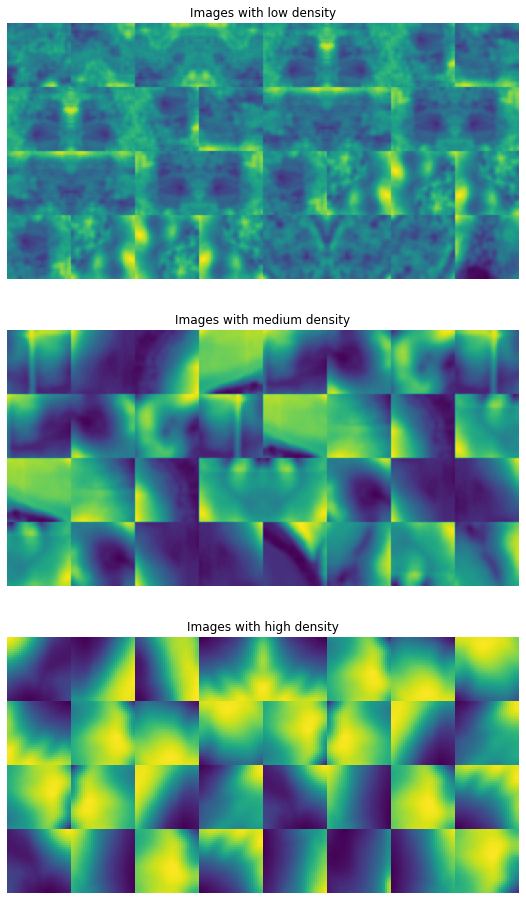
These images help us understand the representation that the model has learned. In the top panel, we see that the images with the lowest probability are those with a lot of “fuzziness”; these are images with lots of noisy LiDAR reflections due to water and vegetation. Since this is effectively random noise, it isn’t possible to predict perfectly what these values will be.
Images with high density, on the other hand, show smoothly varying topography and very strong spatial autocorrelations. Again, this isn’t terribly surprising because the model has favored data points for which it can easily yield very good pixel-level predictions. If each pixel differs from its neighbor by only a small amount, it is much easier to construct a predictive model with low error.
I hope that this provided a straightforward and minimal example of how to use Tensorflow Probability for a rather sophisticated machine learning task. I’ve been impressed with the functionality incorporated into the TFP codebase and look forward to using it more in the future!