Creating an emulator for an agent-based model
Published:
Computers are (still) getting faster every year and it is now commonplace to run simulations in seconds that would have required hours’ or days’ worth of compute time in previous generations. That said, we still often come across cases where our computer models are simply too intricate and/or have too many components to run as often and quickly as we would like. In this scenario, we are frequently forced to choose a limited subset of potential scenarios manifest as parameter settings for which we have the resources to run simulations. I’ve written this notebook to show how to use a statistical emulator to help understand how the outputs of a model’s simulations might vary with parameters.
This is going to be similar in many ways to the paper written by Kennedy and O’Hagan (2001) which is frequently cited on the subject, though our approach will be simpler in some regards.To start us off, I’ve modified an example of an agent-based model for disease spread on a grid which was written by Damien Farrell on his personal site. We’re going to write a statistical emulator in PyMC3 and use it to infer likely values for the date of peak infection without running the simulator exhaustively over the entire parameter space.
TL;DR: we run our simulation for a few combinations of parameter settings and then try to estimate a simulation summary statistic for the entire parameter space.
If you’re interested in reproducing this notebook, you can find the abm_lib.py file at this gist.
from abm_lib import SIR
import time
from tqdm import tqdm

%config InlineBackend.figure_format = 'retina'
Simulating with an ABM
We’ll first need to specify the parameters for the SIR model. This model is fairly rudimentary and is parameterized by:
- The number of agents in the simulation
- The height and width of the spatial grid
- The proportion of infected agents at the beginng
- Probability of infecting other agents in the same grid cell
- Probability of dying from the infection
- Mean + standard deviation of time required to overcome the infection and recover
These parameters, as well as the number of timesteps in the simulation, are all specified in the following cells. I am going to let most of the parameters be fixed as single values - only two parameters will be allowed to vary in our simulations.
fixed_params = {
    "N":20000,
    "width":80,
    "height":30,
    "recovery_sd":4,
    "recovery_days":21,
    "p_infected_initial":0.0002
}
For the probability of transmission and death rate, we’ll randomly sample some values from the domains indicated below.
sample_bounds = {
    "ptrans":[0.0001, 0.2],
    "death_rate":[0.001, 0.1],
}
Here, we iteratively sample new values of the parameters and run the simulation. Since each one takes ~40 seconds, it would take too long to run the simulation at every single parameter value in a dense grid of 1000 or more possible settings.
import numpy as np

n_samples_init = 10
input_dicts    = []

for i in range(n_samples_init):
    d = fixed_params.copy()
    for k,v in sample_bounds.items():
        d[k] = np.random.uniform(*v)
    input_dicts += [d]


n_steps=100

simulations = [SIR(n_steps, model_kwargs=d) for d in input_dicts]
all_states  = [x[1] for x in simulations]
100%|██████████| 100/100 [00:57<00:00,  1.75it/s]
100%|██████████| 100/100 [00:36<00:00,  2.78it/s]
100%|██████████| 100/100 [00:52<00:00,  1.91it/s]
100%|██████████| 100/100 [00:35<00:00,  2.80it/s]
100%|██████████| 100/100 [00:37<00:00,  2.64it/s]
100%|██████████| 100/100 [00:40<00:00,  2.48it/s]
100%|██████████| 100/100 [00:40<00:00,  2.47it/s]
100%|██████████| 100/100 [00:40<00:00,  2.44it/s]
100%|██████████| 100/100 [00:39<00:00,  2.50it/s]
100%|██████████| 100/100 [00:23<00:00,  4.32it/s]
Next, we combine all the sampled parameter values into a dataframe. We also add a column for our response variable which presents a summary of the results from the ABM simulation. We’ll use the timestep for which the level of infection was highest as the worst_day column in the dataframe.
import pandas as pd

params_df = pd.DataFrame(input_dicts)

# Add column showing the day with the peak infection rate
params_df['worst_day'] = [np.argmax(x[...,1].sum(axis=(1,2))) for x in all_states]
We can also spit out a few animations to visualize how the model dynamics behave. This can take quite awhile, however.
import matplotlib.gridspec as gridspec
import matplotlib.pyplot as plt
from mpl_toolkits.axes_grid1 import make_axes_locatable

generate_animations = False
figure_directory = './figures/sir-states/'

if generate_animations:
    colors=['r','g','b']
    for k, pair in enumerate(simulations):
        model, state = pair
        for i in tqdm(range(n_steps)):
            fig = plt.figure(constrained_layout=True, figsize=(10,2))
            gs = gridspec.GridSpec(ncols=4, nrows=1, figure=fig)
            ax = fig.add_subplot(gs[2:4])
            im = ax.imshow(state[i,:,:,1].T, vmax=20, vmin=0, cmap='jet')
            ax.set_axis_off()
            divider = make_axes_locatable(ax)
            cax = divider.append_axes("right", size="3%", pad=0.05)
            plt.colorbar(im, cax=cax, label='Number infected')

            ax2 = fig.add_subplot(gs[0:2])
            for j in range(3):
                ax2.plot(state[:,:,:,j].sum(axis=(1,2)), color=colors[j])
                ax2.scatter(i, state[i,:,:,j].sum(), color=colors[j])
            ax2.set_ylabel('Number infected')
            ax2.set_xlabel('Timestep')
            plt.savefig(figure_directory+'frame_{1}_{0}.jpg'.format( str(i).zfill(5),j), bbox_inches='tight', dpi=250)
            plt.close()

        ! cd /Users/v7k/Dropbox\ \(ORNL\)/research/abm-inference/figures/sir-states/; convert *.jpg sir_states{k}.gif; rm *.jpg
Clearly, the model parameters make a major difference in the rate of spread of the virus. In the lower case, the spread requires over 100 timesteps to infect most of the agents.
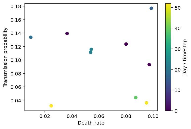
If we make a plot depicting the date of peak infection as a function of ptrans and death_rate, we’ll get something that looks like the picture below. This is a fairly small set of points and the rest of this notebook will focus on interpolating between them in a way which provides quantified uncertainty.
plt.scatter(params_df.death_rate, params_df.ptrans, c=params_df.worst_day)
plt.xlabel('Death rate'), plt.ylabel('Transmission probability'), plt.colorbar(label="Day / timestep");
Building a simplified Gaussian process emulator
Our probabilistic model for interpolating between ABM parameter points is shown below in the next few code cells. We first rescale the parameter points and the response variable to have unit variance. This makes it a little easier to specify reasonable priors for the parameters of our Gaussian process model.
param_scales  = params_df.std()
params_df_std = params_df / param_scales

input_vars = list(sample_bounds.keys())
n_inputs   = len(input_vars)
We assume that the mean function of our Gaussian process is a constant, and we use fairly standard priors for the remaining GP parameters. In particular, we use a Matern52 covariance kernel which allows the correlation between values of our response variable to be a function of the Euclidean distance between them.
import pymc3 as pm

def sample_emulator_model_basic(X, y, sampler_kwargs={'target_accept':0.95}):
    _, n_inputs = X.shape

    with pm.Model() as emulator_model:
        intercept    = pm.Normal('intercept', sd=20)
        length_scale = pm.HalfNormal('length_scale', sd=3)
        variance     = pm.InverseGamma('variance', alpha=0.1, beta=0.1)

        cov_func     = variance*pm.gp.cov.Matern52(n_inputs, ls=length_scale)
        mean_func    = pm.gp.mean.Constant(intercept)

        gp       = pm.gp.Marginal(mean_func=mean_func, cov_func=cov_func)
        noise    = pm.HalfNormal('noise')
        response = gp.marginal_likelihood('response', X, y, noise)
        trace    = pm.sample(**sampler_kwargs)

    return trace, emulator_model, gp
Fitting the model runs fairly quickly since we have only a handful of observed data points. If we had 1000 or more instead of 10, we might need to use a different flavor of Gaussian process model to accommodate the larger set of data.
X = params_df_std[input_vars].values
y = params_df_std['worst_day'].values

trace, emulator_model, gp = sample_emulator_model_basic(X, y)
<ipython-input-15-996f43c1af4e>:17: FutureWarning: In v4.0, pm.sample will return an `arviz.InferenceData` object instead of a `MultiTrace` by default. You can pass return_inferencedata=True or return_inferencedata=False to be safe and silence this warning.
  trace    = pm.sample(**sampler_kwargs)
Auto-assigning NUTS sampler...
Initializing NUTS using jitter+adapt_diag...
Multiprocess sampling (4 chains in 4 jobs)
NUTS: [noise, variance, length_scale, intercept]
Sampling 4 chains for 1_000 tune and 1_000 draw iterations (4_000 + 4_000 draws total) took 30 seconds.
The number of effective samples is smaller than 25% for some parameters.
Predicting at new locations is easy too, once we have our fitted model.
Xnew = np.asarray(np.meshgrid(*[np.linspace(*sample_bounds[k]) for k in input_vars]))
Xnew = np.asarray([Xnew[0].ravel(), Xnew[1].ravel()]).T / param_scales[input_vars].values

with emulator_model:
    pred_mean, pred_var = gp.predict(Xnew, given=trace, diag=True)
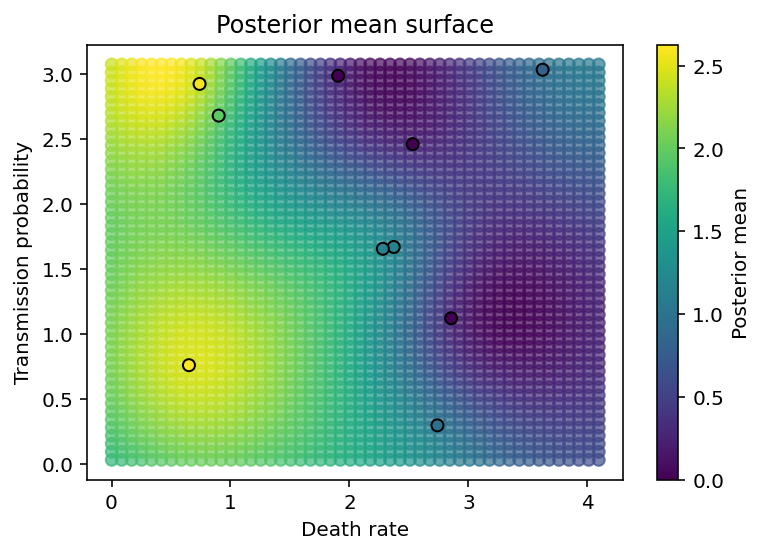
The final two cells create plots showing the posterior predictive distribution of the GP over all the values in parameter space for which we have no data. As we can see, it smoothly interpolates between data points.
plt.figure(figsize=(6,4))
plt.scatter(Xnew[:,0], Xnew[:,1], c=pred_mean, alpha=0.7)
plt.scatter(X[:,0], X[:,1], c=y, edgecolor='k')
plt.xlabel('Death rate'), plt.ylabel('Transmission probability'),
plt.colorbar(label='Posterior mean'), plt.title('Posterior mean surface');
(<matplotlib.colorbar.Colorbar at 0x7fd2c3beb3a0>,
 Text(0.5, 1.0, 'Posterior mean surface'))
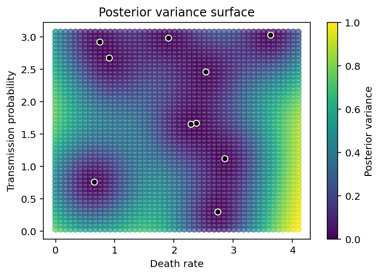
We also see that the variance in the predictions grows as we move farther and farther away from observed data points.
plt.figure(figsize=(6,4))
plt.scatter(Xnew[:,0], Xnew[:,1], c=pred_var, alpha=0.7)
plt.scatter(X[:,0], X[:,1], color='k', edgecolor='w')
plt.xlabel('Death rate'), plt.ylabel('Transmission probability'),
plt.colorbar(label='Posterior variance'), plt.title('Posterior variance surface');