To my junior collaborators, this is how I want you to write your research code
An example notebook for creating a geospatial machine learning dataset with opinionated commentary.
As a former grad student employed in tech, I am well aware of the existing stereotypes of folks with advanced degrees - they aren’t team players, they use poor practices, they’re overly focused on technical aspects, etc. I personally think that my career is an excellent example of all of these.
However, I can give you a strong selling point for people like me as candidates in software development (applicable mostly in the USA, where 5 year+ PhD programs are the norm).
The point is this: there is no other structured program on the planet that forces so many smart, motivated people to come back to their terrible old codebase and have to deal with it alone, without any help, and with virtually zero budget.
In the best case scenario, you do a bunch of awesome research, submit it for journals and conferences, and 6-12 months later, you have to dig into it again to address peer review comments. In the worst case, your research gets dragged along for years for a variety of reasons including, but not limited to, (1) personal indifference and apathy, (2) slow review cycles, (3) life, death, birth, and all other acts of chance. I have had projects limp along for four or even five years, requiring me to exhume the code, fix all of the broken dependencies, track down any required data artifacts, and get it running again.
In this document, I will show you some good practices on building a data cleaning script for an ML project using remotely sensed data of Earth’s surface. In some ways, this kind of work it is easy because image data is nice and Numpy is awesome. In other ways, it sucks massively thanks to the curvature of Earth’s surface and the abundance of ways to trip yourself up working in both flat and curvilinear coordinate systems. We’ll download land cover data, which represents the continental USA as a grid of pixels across roughly 15 classes like forest, grassland, and developed area. We will also overlay this with elevation maps from the NASA’s SRTM data product.
Note: If you want to run the code in this notebook, you’ll need to download the 2021 National Land Cover Dataset from here.
1. Imports
You may think this part is trivial, but there are still ways to make your life miserable. Managing package versions in Python is hard, for structural reasons related to the Python ecosystem. The ecosystem’s greatest strength is its diversity, but this is also the cause of a highly fractured landscape of solutions (pip, conda, uv, poetry, to name a few).
Here’s an idea I will bring up repeatedly in this notebook: your goal is maximize the probability that your future self can reproduce your work and edit it at a much later stage. With this in mind, note the following:
-
Just use
pipwith a virtual environment. You can use a fancy, richly-featured package manager like Poetry. This will make you look like a smart guy when people are looking at your repo. However, be honest with yourself. How likely is it that you are going to be using the same Python tooling in 5 years? My advice is to just usepipwith a virtual environment. It’ll be way slower thanuvand it won’t have as many features as Poetry, but you can be sure that when you dig your code out, you will remember how to dopython -m venv venv && source venv/bin/activate && pip install -r requirements. You might not even be working in tech several years out, in which case you will definitely not want something fancy and richly-featured for the advanced Python developer -
Once you are done with the first pass on your project, run
pip freeze | requirements.txtto automatically pin your dependencies. This has one major downside, namely that you cannot figure out which packages are essential just by looking at the requirements file. If you decide you want to upgrade your code with a nice few feature, you will have to figure out which packages need to be unpinned. Here’s what I would do: after running pip freeze, pass the whole thing to ChatGPT along with your imports and tell it to filter out any modules that aren’t directly imported by your code.
import cv2
import elevation
import geopandas as gpd
import logging
import matplotlib.patches as mpatches
import matplotlib.pyplot as plt
import multiprocessing as mp
import numpy as np
import os
import pandas as pd
import psutil
import rasterio

from dataclasses import dataclass
from functools import partial
from pathlib import Path
from pyproj import CRS, Transformer
from scipy.stats import mode
from shapely.geometry import box
from tqdm.notebook import tqdm
from typing import Tuple

%load_ext watermark
%watermark -iv
matplotlib: 3.9.2
pandas    : 2.2.3
tqdm      : 4.66.5
elevation : 1.1.3
pyproj    : 3.7.0
geopandas : 0.13.2
logging   : 0.5.1.2
cv2       : 4.10.0
numpy     : 1.26.4
scipy     : 1.14.1
rasterio  : 1.3.11
shapely   : 2.0.6
psutil    : 6.1.0
2. Setting up the config
You may want to put your configs in a JSON or a YAML. This is a terrible idea. I’ve tried both and hated both ways. The main issue is that putting the configs in a separate file makes it at least 2x slower to make a change or edit. It also means that you can shoot yourself in the foot by mishandling type conversion / loading. It also subtly encourages you to make bad configuration specs because you don’t have the full set of objects available in standard Python. Some of these types are really quite helpful.
Just use a dataclass instead. I especially like using pathlib to set any file paths ahead of time in an easily readable way.
Feel free to make this sucker as long as it needs to be. If you’re feeling really paranoid, you can even add validators like shown below.
You might think that the validation function here is overkill, and that even the lowest imbecile wouldn’t make the mistake of specifying a set of invalid lat/long coordinates. Just keep in mind that more successful your project is, the more edits you’ll need to make to it to accommodate the more and more grandiose objectives you’ll come up with. Eventually, you will do something dumb. Catch it early and don’t let it propagate into your expensive computation cells later.
current_path = Path.cwd()


@dataclass
class Config:
    logging_level = logging.INFO

    # Data paths
    data_dir: Path = current_path / 'data'
    nlcd_path: Path = data_dir / 'nlcd_2021_land_cover_l48_20230630.img' # Make sure you have this file before you start
    output_path_train: Path = data_dir / 'train.npy'
    output_path_test: Path = data_dir / 'test.npy'
    split_save_path: Path = data_dir / "split.gpkg"

    # Geographic bounds (WGS84 coordinates)
    # bbox_west: float = -116.2
    # bbox_east: float = -106.34
    # bbox_south: float = 30.9
    # bbox_north: float = 44.2
    bbox_west: float = -119.0
    bbox_east: float = -64.0
    bbox_south: float = 22.0
    bbox_north: float = 49.0


    # Sampling parameters
    image_size: int = 40  # Size of output images
    meters_per_raw_pixel: float = 30.0  # Meters per pixel in the raw data
    downsample_ratio: int = 2  # Downsampling factor
    max_fraction_reject_class: float = 0.9  # Maximum fraction of pixels allowed in a reject-eligible class
    area_fraction_test: float = 0.2  # Fraction of area to reserve for testing
    n_grid_unit: int = 50  # discrete units in each dimension for gridding the domain into discrete units

    # Processing parameters
    random_seed: int = 827  # Random seed for reproducibility
    recompute_counts: bool = False  # Whether to recompute class counts
    show_plots: bool = True  # Whether to display plots

    # CRS parameters
    working_crs: str = 'EPSG:4326'  # CRS for geographic operations (WGS84)

    nlcd_original_classes_for_reject = {11}
    nlcd_original_unknown_class = 0

    # Parameters for DEM processing
    dem_nodata_threshold: float = 0.25
    dem_product: str = 'SRTM1' # Choices are 'SRTM1' or 'SRTM3', lower resolution
    download_dem: bool = False

    # Mapping from raw NLCD classes to RGB colors for visualization
    nlcd_to_rgb  = {
            11: (0.278, 0.420, 0.627),
            12: (0.820, 0.867, 0.976),
            21: (0.867, 0.788, 0.788),
            22: (0.847, 0.576, 0.510),
            23: (0.929, 0.0, 0.0),
            24: (0.667, 0.0, 0.0),
            31: (0.698, 0.678, 0.639),
            41: (0.408, 0.667, 0.388),
            42: (0.110, 0.388, 0.188),
            43: (0.710, 0.788, 0.557),
            51: (0.647, 0.549, 0.188),
            52: (0.800, 0.729, 0.486),
            71: (0.886, 0.886, 0.757),
            72: (0.788, 0.788, 0.467),
            73: (0.600, 0.757, 0.278),
            74: (0.467, 0.678, 0.576),
            81: (0.859, 0.847, 0.239),
            82: (0.667, 0.439, 0.157),
            90: (0.729, 0.847, 0.918),
            95: (0.439, 0.639, 0.729),
        }
    nlcd_to_name = {
        11: "Open Water",
        12: "Perennial Ice/Snow",
        21: "Developed, Open Space",
        22: "Developed, Low Intensity",
        23: "Developed, Medium Intensity",
        24: "Developed, High Intensity",
        31: "Barren Land (Rock/Sand/Clay)",
        41: "Deciduous Forest",
        42: "Evergreen Forest",
        43: "Mixed Forest",
        51: "Dwarf Scrub",
        52: "Shrub/Scrub",
        71: "Grassland/Herbaceous",
        72: "Sedge/Herbaceous",
        73: "Lichens",
        74: "Moss",
        81: "Pasture/Hay",
        82: "Cultivated Crops",
        90: "Woody Wetlands",
        95: "Emergent Herbaceous Wetlands"
    }

    def __post_init__(self):
        # Validate bbox coordinates
        if not (self.bbox_west < self.bbox_east):
            raise ValueError(f"Invalid bbox coordinates: bbox_west ({self.bbox_west}) should be less than bbox_east ({self.bbox_east})")
        if not (self.bbox_south < self.bbox_north):
            raise ValueError(f"Invalid bbox coordinates: bbox_south ({self.bbox_south}) should be less than bbox_north ({self.bbox_north})")

        # Validate file paths
        if not self.nlcd_path.is_file():
            raise FileNotFoundError(f"NLCD file not found at {self.nlcd_path}")
        if not self.data_dir.is_dir():
            raise FileNotFoundError(f"Data directory not found at {self.data_dir}")


config = Config()

logging.basicConfig(
    format='[%(levelname)s] %(message)s',
    level=config.logging_level,
)

np.random.seed(827)

logging.info(f"Setting project data directory to {config.data_dir}")
[INFO] Setting project data directory to /mnt/m2ssd/data/Dropbox/research/nlcd-inpaint/generative-land-cover/data
You should also use logging extensively with Jupyter notebooks. It’s just as easy as using print. I like to use INFO for anything remotely resembling a distinct conceptual step in the pipeline. For any row-level operations, i.e. anything inside a for-loop with more than 5 iterates, I’ll use DEBUG.
3. Dataset Information and CRS Setup
This is where the true fun begins. With your biggest data files, print out everything before you start working. For commonly used Python libraries, ChatGPT and Sonnet are perfectly capable of getting all of the metadata fields you never knew about. See below for an example.
When you see a kwarg like always_xy, you know that someone got really upset at some point.
Here’s a piece of advice for any kind of geographic data analysis: if, at any point in time, you do not know with 100% certainty whether an imported module or function is using a (lat,long) or (long,lat) convention for ordering of coordinates, you should just stop, take a deep breath, and read the docs.
# Open the NLCD dataset and print basic information
with rasterio.open(config.nlcd_path) as src:
    logging.info(f"Dataset CRS: {src.crs}")
    logging.info(f"Dataset bounds: {src.bounds}")
    logging.info(f"Dataset shape: {src.shape}")
    logging.info(f"Dataset resolution: {src.res}")
    logging.info(f"Dataset transform: {src.transform}")

    # Set up CRS transformers
    data_crs = src.crs
    working_crs = CRS.from_string(config.working_crs)

    # Create transformers for converting between CRS
    to_working_crs = Transformer.from_crs(data_crs, working_crs, always_xy=True)
    from_working_crs = Transformer.from_crs(working_crs, data_crs, always_xy=True)

    # Convert dataset bounds to working CRS for validation
    bounds = src.bounds
    ds_left, ds_bottom = to_working_crs.transform(bounds.left, bounds.bottom)
    ds_right, ds_top = to_working_crs.transform(bounds.right, bounds.top)


    logging.info("\nBounding box validation:")
    logging.info(f"Dataset bounds (lon/lat): {ds_left:.4f}, {ds_bottom:.4f}, {ds_right:.4f}, {ds_top:.4f}")
    logging.info(f"Selected bbox (lon/lat): {config.bbox_west}, {config.bbox_south}, {config.bbox_east}, {config.bbox_north}")
    samples_x = src.shape[1] / config.downsample_ratio / config.image_size
    samples_y = src.shape[0] / config.downsample_ratio / config.image_size

    logging.info(f"Maximum number of sampled images from full dataset: {samples_x * samples_y:.0f}")
[INFO] Dataset CRS: PROJCS["Albers_Conical_Equal_Area",GEOGCS["WGS 84",DATUM["WGS_1984",SPHEROID["WGS 84",6378137,298.257223563,AUTHORITY["EPSG","7030"]],AUTHORITY["EPSG","6326"]],PRIMEM["Greenwich",0,AUTHORITY["EPSG","8901"]],UNIT["degree",0.0174532925199433,AUTHORITY["EPSG","9122"]],AUTHORITY["EPSG","4326"]],PROJECTION["Albers_Conic_Equal_Area"],PARAMETER["latitude_of_center",23],PARAMETER["longitude_of_center",-96],PARAMETER["standard_parallel_1",29.5],PARAMETER["standard_parallel_2",45.5],PARAMETER["false_easting",0],PARAMETER["false_northing",0],UNIT["meters",1],AXIS["Easting",EAST],AXIS["Northing",NORTH]]
[INFO] Dataset bounds: BoundingBox(left=-2493045.0, bottom=177285.0, right=2342655.0, top=3310005.0)
[INFO] Dataset shape: (104424, 161190)
[INFO] Dataset resolution: (30.0, 30.0)
[INFO] Dataset transform: | 30.00, 0.00,-2493045.00|
| 0.00,-30.00, 3310005.00|
| 0.00, 0.00, 1.00|
[INFO]
Bounding box validation:
[INFO] Dataset bounds (lon/lat): -119.7861, 21.7423, -63.6722, 49.1771
[INFO] Selected bbox (lon/lat): -119.0, 22.0, -64.0, 49.0
[INFO] Maximum number of sampled images from full dataset: 2630016
4. Class Counting and Mapping
# Function to compute class counts in a block
def compute_block_counts(data):
    unique, counts = np.unique(data, return_counts=True)
    return dict(zip(unique, counts))

# Calculate available memory
available_memory = psutil.virtual_memory().available
dtype_size = np.dtype('uint8').itemsize
max_elements = available_memory // (2 * dtype_size)  # Use half of available memory

if not config.recompute_counts:
    logging.info(f"Skipping class counts computation from raster; loading from file")
else:
    with rasterio.open(config.nlcd_path) as src:
        # Convert bbox to pixel coordinates
        bbox_left, bbox_bottom = from_working_crs.transform(config.bbox_west, config.bbox_south)
        bbox_right, bbox_top = from_working_crs.transform(config.bbox_east, config.bbox_north)

        # Get pixel bounds
        row_start, col_start = src.index(bbox_left, bbox_top)
        row_end, col_end = src.index(bbox_right, bbox_bottom)

        # Ensure correct order
        row_start, row_end = min(row_start, row_end), max(row_start, row_end)
        col_start, col_end = min(col_start, col_end), max(col_start, col_end)

        # Calculate block size for the bbox region
        bbox_height = row_end - row_start
        bbox_width = col_end - col_start
        total_pixels = bbox_height * bbox_width
        n_blocks = max(1, total_pixels // max_elements)
        block_height = bbox_height // n_blocks

        # Initialize counts dictionary
        total_counts = {}

        # Process data in blocks within the bbox
        for i in tqdm(range(row_start, row_end, block_height), desc='Computing class counts'):
            # Read a block of data
            window = rasterio.windows.Window(
                col_start, i,
                col_end - col_start,
                min(block_height, row_end - i)
            )
            data = src.read(1, window=window)

            # Update counts
            block_counts = compute_block_counts(data)
            for k, v in block_counts.items():
                total_counts[k] = total_counts.get(k, 0) + v

    logging.info(f"Unique values present in the bbox: {len(total_counts)}: {total_counts.keys()}")

    # Drop the counts which are in class 0 (Unknown)
    _ = total_counts.pop(config.nlcd_original_unknown_class, None)
[INFO] Skipping class counts computation from raster; loading from file
if not config.recompute_counts:
    logging.info(f"Skipping class counts computation from raster; loading from file")
    classes_df = pd.read_parquet(Path(config.data_dir) / 'class_distribution.parquet')
    total_counts = classes_df.set_index('class_value')['count'].to_dict()
    classes_df['RGB'] = classes_df['class_value'].map(config.nlcd_to_rgb)


else:
# Convert to DataFrame for better visualization
    classes_df = pd.DataFrame([
        {'class_value': k, 'count': v, 'name': config.nlcd_to_name.get(k, 'Unknown')}
        for k, v in total_counts.items()
    ])
    classes_df['percentage'] = classes_df['count'] / classes_df['count'].sum() * 100
    classes_df = classes_df.sort_values('count', ascending=False)

    # Rename the index (currently unnamed) to "class"
    classes_df.index.name = 'class'
    classes_df = classes_df.sort_index()

    # Load the mapping from original class codes to RGB for plotting and add to the dataframe
    # We will use these for plotting later
    classes_df['RGB'] = classes_df['class_value'].map(config.nlcd_to_rgb)
    classes_df.to_parquet(Path(config.data_dir) / 'class_distribution.parquet')
    present_classes = sorted(total_counts.keys())

class_mapping = classes_df['class_value'].reset_index(drop=True).reset_index().set_index('class_value')['index'].to_dict()
reverse_mapping = {idx: old_val for old_val, idx in class_mapping.items()}

palette_series = classes_df['RGB']
lut = np.array(palette_series.tolist())
logging.info(f"Prepare lookup table for plotting with shape {lut.shape}")

# Print mapping from original classes to zero-based indices
logging.info("\nClass mapping:")
logging.info(class_mapping)
[INFO] Skipping class counts computation from raster; loading from file
[INFO] Prepare lookup table for plotting with shape (16, 3)
[INFO]
Class mapping:
[INFO] {11: 0, 12: 1, 21: 2, 22: 3, 23: 4, 24: 5, 31: 6, 41: 7, 42: 8, 43: 9, 52: 10, 71: 11, 81: 12, 82: 13, 90: 14, 95: 15}
Creating a test/train split
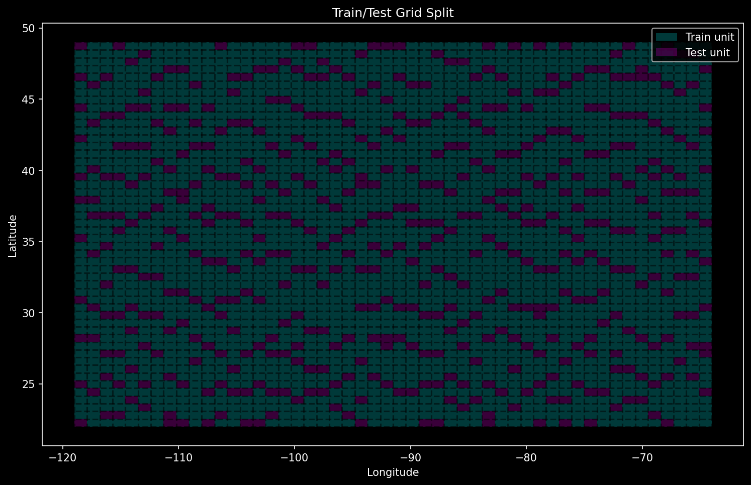
For a good analysis, you need to make sure that there is no data leakage from test or validation into training. In a geospatial context, this means that the spatial overlap between the areas used for each split should be zero. Here, we split up the entire domain into grid cells and pick some of them to be test units.
If you need to perform some sort of random sampling like for training and test units, just use quasi-Monte Carlo (QMC) via something like the Sobel method. QMC is generally applicable in most cases where you would use Monte Carlo, and you can generally get more visually pleasing pseudorandom assortments of points with it. It also makes you seem smart, which is invaluable in peer review.
from scipy.stats import qmc  # Built into scipy, no extra installation needed

# Set up grid for train/test split
with rasterio.open(config.nlcd_path) as src:
    # Create grid cells in working CRS using bbox
    x_edges = np.linspace(config.bbox_west, config.bbox_east, config.n_grid_unit + 1)
    y_edges = np.linspace(config.bbox_south, config.bbox_north, config.n_grid_unit + 1)

    # Create grid cell polygons
    grid_cells = []
    for i in range(len(x_edges)-1):
        for j in range(len(y_edges)-1):
            # Create polygon in working CRS
            polygon = {
                'geometry': {
                    'type': 'Polygon',
                    'coordinates': [[
                        [x_edges[i], y_edges[j]],
                        [x_edges[i+1], y_edges[j]],
                        [x_edges[i+1], y_edges[j+1]],
                        [x_edges[i], y_edges[j+1]],
                        [x_edges[i], y_edges[j]]
                    ]]
                },
                'properties': {'id': len(grid_cells)}
            }
            grid_cells.append(polygon)

    # Create GeoDataFrame in working CRS
    grid_gdf = gpd.GeoDataFrame.from_features(grid_cells, crs=working_crs)

    # Set up Sobol sequence generator
    n_cells = len(grid_gdf)
    n_test = int(n_cells * config.area_fraction_test)

    # Generate Sobol sequence and scale to unique grid indices
    sobol_points = qmc.Sobol(d=1, seed=config.random_seed).random(n=n_test)
    sobol_indices = (sobol_points.flatten() * (n_cells - 1)).astype(int)
    sobol_indices = np.unique(sobol_indices)

    # If we got fewer unique indices than needed, add random ones
    if len(sobol_indices) < n_test:
        additional_indices = np.random.choice(
            np.setdiff1d(np.arange(n_cells), sobol_indices),
            size=n_test - len(sobol_indices),
            replace=False
        )
        sobol_indices = np.concatenate([sobol_indices, additional_indices])

    # Assign splits
    grid_gdf['split'] = 'train'
    grid_gdf.loc[sobol_indices, 'split'] = 'test'
    logging.info(f"Generated {n_test} test cells out of {n_cells} total cells and saved to grid_gdf")

# Save the grid to a GeoPackage file
grid_gdf.to_file(config.split_save_path, driver='GPKG')
logging.info(f"Saved geodataframe for grid of train/test cells to {config.split_save_path}")

if config.show_plots:
    fig, ax = plt.subplots(figsize=(12, 8))
    grid_gdf[grid_gdf['split'] == 'train'].plot(ax=ax, color='c', alpha=0.3)
    grid_gdf[grid_gdf['split'] == 'test'].plot(ax=ax, color='m', alpha=0.3)

    for x in x_edges:
        ax.axvline(x, color='black', linestyle='--', alpha=0.5)
    for y in y_edges:
        ax.axhline(y, color='black', linestyle='--', alpha=0.5)

    # Manually create legend elements
    legend_elements = [
        mpatches.Patch(facecolor='c', alpha=0.3, label='Train unit'),
        mpatches.Patch(facecolor='m', alpha=0.3, label='Test unit')
    ]
    ax.legend(handles=legend_elements, loc='best')

    ax.set_title('Train/Test Grid Split')
    ax.set_xlabel('Longitude')
    ax.set_ylabel('Latitude')
    plt.show()
/mnt/m2ssd/data/Dropbox/research/nlcd-inpaint/.venv/lib/python3.10/site-packages/scipy/stats/_qmc.py:958: UserWarning: The balance properties of Sobol' points require n to be a power of 2.
  sample = self._random(n, workers=workers)
[INFO] Generated 500 test cells out of 2500 total cells and saved to grid_gdf
[INFO] Saved geodataframe for grid of train/test cells to /mnt/m2ssd/data/Dropbox/research/nlcd-inpaint/generative-land-cover/data/split.gpkg
6. Sampling Land Cover Images
At this point, I start to have controversial opinions.
I don’t care if the Jupyter cells are too long. It just doesn’t bother me. I don’t think these functions belong in a separate .py file. Why? Because I ultimately think that reproducible research should have a linear representation, and anything that messes with this mental map of the whole thing as just a top-to-bottom execution is bad.
A corollary to this is that it is most helpful if you can anchor your understanding of a notebook with many long code cells by forming landmark visual outputs or tables that help your brain remember where everything happens. I’m a huge fan of animations for this purpose.
Another opinion of mine is that getting cute with optimizing vectorized functions is helpful if you are running your code many times a day, but less so if it’s just a one-time thing. Nested loops are bad form in scientific programming in Python, but I’d rather be able to go back and actually understand what is happening.
I can write a way more performant version of the code below using vectorized Numpy functions and liberal usage of Numba’s JIT. I take relish in having done this before.
I also know that I am too stupid to be able to quickly refresh myself on how an optimal implementation of this works, six months later. Be brave enough to embrace the limits of your own mind. What you see below is a bit of a local optimum between my impatience with slow code and my deep, deep fear of not remembering how any of this works.
There’s another cute thing I could do. If you look closely, you can tell that this code is really just splitting up my spatial domain into adjacent, mutually disjoint rectangular subsets. Much of this could be done by reading a large block of raster and doing .reshape on it to go from (10000,10000) to (1_000_000, 10, 10) or similar dimensions. However, this means that I would need to form the bounding box for each image post-hoc by trying to figure out which coordinates were used by each piece of the image.
Again, this is where I know I can make some mistakes leading to nasty, hard-to-pin-down errors later, so I just do the dumb option and let myself sleep at night.
Run the slow code and go buy yourself a nice piece of chocolate cake at the grocery store while it finishes.
def downsample_patch(patch: np.ndarray, ratio: int) -> np.ndarray:
    """Downsample a patch by taking the mode of each ratio x ratio window."""
    if ratio == 1:
        return patch

    # Reshape into blocks of size ratio x ratio
    h, w = patch.shape
    new_h, new_w = h // ratio, w // ratio
    reshaped = patch.reshape(new_h, ratio, new_w, ratio)

    # Move the two ratio axes adjacent so each block becomes one dimension
    # resulting shape: (new_h * new_w, ratio * ratio)
    reshaped = reshaped.swapaxes(1, 2).reshape(new_h * new_w, ratio * ratio)

    # mode(..., axis=1) finds the most frequent value in each row
    block_modes, _ = mode(reshaped, axis=1)

    # Reshape back to (new_h, new_w)
    downsampled = block_modes.reshape(new_h, new_w)

    return downsampled

def get_pixel_bounds(src, x: float, y: float, size_pixels: int) -> Tuple[slice, slice]:
    """Convert geographic coordinates to pixel bounds for image extraction."""
    # Convert from working CRS to data CRS
    x_data, y_data = from_working_crs.transform(x, y)

    # Convert to pixel coordinates
    row, col = src.index(x_data, y_data)

    # Calculate pixel bounds
    half_size = size_pixels // 2
    row_start = row - half_size
    row_end = row + half_size
    col_start = col - half_size
    col_end = col + half_size

    return (slice(row_start, row_end), slice(col_start, col_end))

def check_overlap(point_coords: Tuple[float, float], image_size_meters: float,
                 grid_gdf: gpd.GeoDataFrame, split: str) -> bool:
    """Check if an image centered at point_coords overlaps with the specified split area."""
    x, y = point_coords
    half_size = image_size_meters / 2

    # Create a box representing the image extent in working CRS
    image_box = box(x - half_size, y - half_size,
                   x + half_size, y + half_size)

    # Check intersection with grid cells of the opposite split
    opposite_split = 'test' if split == 'train' else 'train'
    opposite_cells = grid_gdf[grid_gdf['split'] == opposite_split]

    return not any(image_box.intersects(cell) for cell in opposite_cells.geometry)

def is_within_bbox(x: float, y: float) -> bool:
    """Check if a point is within the specified bbox."""
    return (config.bbox_west <= x <= config.bbox_east and
            config.bbox_south <= y <= config.bbox_north)

def process_cell(cell_data, args):
    """Process a single cell of data.

    Args:
        cell_data: tuple of (cell, src_bounds, src_res, transforms)
        args: dict containing configuration parameters
    """
    cell, src_bounds, src_res, transforms = cell_data
    to_working_crs, from_working_crs = transforms

    # Unpack configuration
    config = args['config']
    class_mapping = args['class_mapping']
    full_size_pixels = config.image_size * config.downsample_ratio

    bounds = cell.geometry.bounds
    split = cell['split']

    # Convert bounds to pixel coordinates
    bbox_left, bbox_bottom = from_working_crs.transform(bounds[0], bounds[1])
    bbox_right, bbox_top = from_working_crs.transform(bounds[2], bounds[3])

    with rasterio.open(config.nlcd_path) as src:
        row_start, col_start = src.index(bbox_left, bbox_top)
        row_end, col_end = src.index(bbox_right, bbox_bottom)

        # Ensure correct order
        row_start, row_end = min(row_start, row_end), max(row_start, row_end)
        col_start, col_end = min(col_start, col_end), max(col_start, col_end)

        # Read the entire cell into memory
        cell_data = src.read(1, window=rasterio.windows.Window(
            col_start, row_start,
            col_end - col_start,
            row_end - row_start
        ))

    results = []

    # Extract images from the cell
    for i in range(0, cell_data.shape[0] - full_size_pixels + 1, full_size_pixels):
        for j in range(0, cell_data.shape[1] - full_size_pixels + 1, full_size_pixels):
            patch = cell_data[i:i + full_size_pixels, j:j + full_size_pixels]

            # Reject if any pixels are unknown
            if np.any(patch == config.nlcd_original_unknown_class):
                continue

            # Check water fraction
            reject = False
            for c in config.nlcd_original_classes_for_reject:
                class_fraction = np.mean(patch == c)
                if class_fraction > config.max_fraction_reject_class:
                    reject = True
                    break
            if reject:
                continue

            # Downsample the patch
            downsampled = downsample_patch(patch, config.downsample_ratio)

            # Create a copy for remapping
            remapped = downsampled.copy()
            # Remap classes to zero-based indices
            for old_val, new_val in class_mapping.items():
                remapped[downsampled == old_val] = new_val

            with rasterio.open(config.nlcd_path) as src:
                x_ul, y_ul = to_working_crs.transform(*src.xy(row_start + i, col_start + j))
                x_lr, y_lr = to_working_crs.transform(*src.xy(
                    row_start + i + full_size_pixels,
                    col_start + j + full_size_pixels
                ))

            bbox = box(x_ul, y_ul, x_lr, y_lr)
            results.append((remapped, bbox, split))

    return results

def sample_images_parallel(grid_gdf, config, class_mapping, n_processes=None) -> tuple:
    """Sample and process images in parallel for either train or test set.

    Args:
        grid_gdf: GeoDataFrame containing grid cells
        config: Configuration object
        class_mapping: Dictionary mapping old class values to new ones
        n_processes: Number of processes to use (defaults to CPU count - 1)

    Returns:
        tuple: (train_images, train_gdf, test_images, test_gdf)
    """
    if n_processes is None:
        n_processes = max(1, mp.cpu_count() - 1)

    # Get source metadata once
    with rasterio.open(config.nlcd_path) as src:
        src_bounds = src.bounds
        src_res = src.res

    # Prepare arguments for parallel processing
    transforms = (to_working_crs, from_working_crs)  # Assuming these are defined
    cell_data = [(cell, src_bounds, src_res, transforms) for _, cell in grid_gdf.iterrows()]

    # Prepare static arguments
    process_args = {
        'config': config,
        'class_mapping': class_mapping
    }

    # Create process pool and process cells in parallel
    logging.info(f"Processing cells using {n_processes} processes...")
    with mp.Pool(n_processes) as pool:
        process_func = partial(process_cell, args=process_args)
        results = list(tqdm(
            pool.imap(process_func, cell_data),
            total=len(cell_data),
            desc="Processing grid cells"
        ))

    # Flatten results and separate train/test
    train_images = []
    test_images = []
    train_bboxes = []
    test_bboxes = []

    for cell_results in results:
        for remapped, bbox, split in cell_results:
            if split == 'train':
                train_images.append(remapped)
                train_bboxes.append(bbox)
            else:
                test_images.append(remapped)
                test_bboxes.append(bbox)

    # Create GeoDataFrames for train and test bounding boxes
    working_crs = grid_gdf.crs  # Get CRS from input GeoDataFrame
    train_gdf = gpd.GeoDataFrame(geometry=train_bboxes, crs=working_crs)
    test_gdf = gpd.GeoDataFrame(geometry=test_bboxes, crs=working_crs)

    return (np.array(train_images), train_gdf, np.array(test_images), test_gdf)


train_images, train_gdf, test_images, test_gdf = sample_images_parallel(
    grid_gdf,
    config,
    class_mapping,
)
Data validation
Coding copilots can do autocomplete a dozen of these assert-type tests in a minute.
Just do them. Do as many as you have patience for.
# Make sure all images are in the valid integer range with no NaNs
assert np.all(np.isfinite(train_images))
assert np.all(np.isfinite(test_images))
logging.info("All images are free of null / NaN values.")

# Make sure in right range of values
assert np.all((train_images >= 0) & (train_images < len(class_mapping))), f"Unqiue train values: {np.unique(train_images)}"
assert np.all((test_images >= 0) & (test_images < len(class_mapping))), f"Unqiue test values: {np.unique(test_images)}"
logging.info("All images are in the correct range of values.")

# Check that the images are the correct size
assert train_images.shape[1:] == (config.image_size, config.image_size), f"Train shape: {train_images.shape} should be {(config.image_size, config.image_size)}"
assert test_images.shape[1:] == (config.image_size, config.image_size), f"Test shape: {test_images.shape}, should be {(config.image_size, config.image_size)}"
logging.info("All images are the correct size.")
[INFO] All images are free of null / NaN values.
[INFO] All images are in the correct range of values.
[INFO] All images are the correct size.
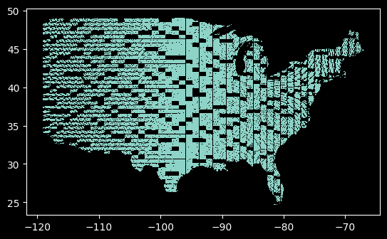
More visual representations of your data are better. Here’s the locations of our sampled images so far. It even has a surprise - the west coast is cut off! It turns out this is a limitation of this data file. Good thing we caught it early!
train_gdf.plot()
<Axes: >
Plot sample images
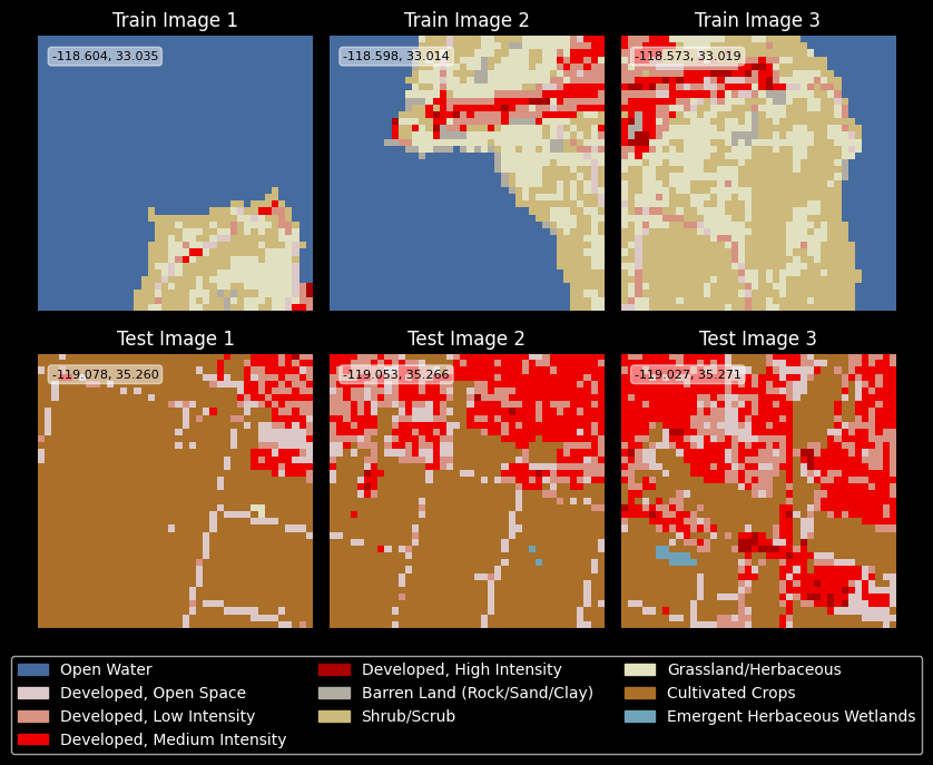
Before, I opted out of doing random sampling of my data and instead decided to partition the entire spatial domain.
A beautiful side effect of this choice is that I can plot the first n examples from both train and test splits, and examine to see if they show continuity from one example to the next. This helps me diagnose subtle indexing errors right away. Fortunately, these appear to be correct.
n_images = 3

seen_classes = set()

if config.show_plots:
    fig, ax = plt.subplots(2, n_images, figsize=(8, 6))

    for i in range(n_images):
        for j, (images, geom, title) in enumerate(zip([train_images, test_images], [train_gdf.iloc[i].geometry, test_gdf.iloc[i].geometry], ["Train", "Test"])):
            ax[j, i].imshow(lut[images[i]])
            ax[j, i].set_title(f"{title} Image {i+1}")
            ax[j, i].axis('off')

            lat, lon = geom.centroid.xy
            ax[j, i].text(1.5, 3, f"{lat[0]:.3f}, {lon[0]:.3f}", color='black', fontsize=8,
                          bbox=dict(facecolor='white', alpha=0.5, boxstyle='round,pad=0.3'))
            seen_classes.update(np.unique(images[i]))

    legend_handles = [mpatches.Patch(color=classes_df.loc[idx, "RGB"], label=classes_df.loc[idx, "name"]) for idx in seen_classes]

    fig.legend(handles=legend_handles, loc='lower center', ncol=3, bbox_to_anchor=(0.5, -0.15))
    plt.tight_layout()
    plt.show()
else:
    logging.info("Skipping display of sample NLCD images. Set `show_plots` to True to display.")
7. Class distribution across sampled images
Paranoia is healthy. I have no reason to believe that the below code will show any discrepancy between the expected sample proportions and the overall marginal distribution of pixels in the original raster file. Yet, we check anyway.
def compute_class_distribution(images):
    unique, counts = np.unique(images, return_counts=True)
    total = counts.sum()
    return {reverse_mapping[cls]: count/total for cls, count in zip(unique, counts)}

train_dist = compute_class_distribution(train_images)
test_dist = compute_class_distribution(test_images)

logging.info("\nFinal class distribution (original class ID: percentage):")
logging.info("\nTraining set:")
for cls_id, pct in train_dist.items():
    logging.info(f"{cls_id} ({config.nlcd_to_name[cls_id]}): {pct*100:.2f}%")
[INFO]
Final class distribution (original class ID: percentage):
[INFO]
Training set:
[INFO] 11 (Open Water): 2.18%
[INFO] 12 (Perennial Ice/Snow): 0.01%
[INFO] 21 (Developed, Open Space): 3.95%
[INFO] 22 (Developed, Low Intensity): 2.00%
[INFO] 23 (Developed, Medium Intensity): 0.99%
[INFO] 24 (Developed, High Intensity): 0.31%
[INFO] 31 (Barren Land (Rock/Sand/Clay)): 0.93%
[INFO] 41 (Deciduous Forest): 11.95%
[INFO] 42 (Evergreen Forest): 10.61%
[INFO] 43 (Mixed Forest): 3.47%
[INFO] 52 (Shrub/Scrub): 19.39%
[INFO] 71 (Grassland/Herbaceous): 12.73%
[INFO] 81 (Pasture/Hay): 7.12%
[INFO] 82 (Cultivated Crops): 17.66%
[INFO] 90 (Woody Wetlands): 5.23%
[INFO] 95 (Emergent Herbaceous Wetlands): 1.48%
8. Downloading and matching with DEM data
Download data using elevation
if config.download_dem:
    n_dem_downloads, bounds = 625, (config.bbox_west, config.bbox_south, config.bbox_east, config.bbox_north)  # should be a square number
    # Define the bounding box for continental USA (approximate)
    # For testing, use a sample pair of values like below:
    # n_dem_downloads, bounds = 4, (-100.0, 28.0, -99.0, 29.0)  # should be a square number

    dem_dir = Path(config.data_dir) / 'dem'
    os.makedirs(dem_dir, exist_ok=True)

    # Calculate the number of splits in each dimension
    n_splits = int(n_dem_downloads ** 0.5)

    # Remove all files from the DEM directory
    for file in dem_dir.glob('*.tif'):
        file.unlink()

    # Split bounds into a grid and download DEM data
    with tqdm(total=n_dem_downloads, desc="Downloading DEM data") as pbar:
        for i in range(n_splits):
            for j in range(n_splits):
                west = bounds[0] + (bounds[2] - bounds[0]) * i / n_splits
                east = bounds[0] + (bounds[2] - bounds[0]) * (i + 1) / n_splits
                south = bounds[1] + (bounds[3] - bounds[1]) * j / n_splits
                north = bounds[1] + (bounds[3] - bounds[1]) * (j + 1) / n_splits

                assert west < east, f"West {west} should be less than east {east}"
                assert south < north, f"South {south} should be less than north {north}"

                dem_save_path = dem_dir / f'conus_dem_{i}_{j}.tif'
                elevation.clip(bounds=(west, south, east, north), output=dem_save_path, product=config.dem_product)

                # Check the statistics on the DEM
                with rasterio.open(dem_save_path) as src:
                    dem_data = src.read(1)
                    dem_nodata = src.nodata
                    dem_stats = {
                        'min': dem_data.min(),
                        'max': dem_data.max(),
                        'mean': dem_data.mean(),
                        'nodata': dem_nodata,
                        'nodata_fraction': np.mean(dem_data == dem_nodata)
                    }
                    logging.info(f"DEM statistics for {dem_save_path}: {dem_stats}")

                pbar.update(1)
else:
    logging.info("Skipping DEM download. Set `download_dem` to True to download.")
Merge into single contiguous DEM raster file
import glob
import os

from rasterio import merge

# Create a list of all the GeoTIFF files
search_pattern = os.path.join(dem_dir, "conus_dem_*.tif")
dem_files = glob.glob(search_pattern)

src_files_to_mosaic = []
for file in dem_files:
    src = rasterio.open(file)
    src_files_to_mosaic.append(src)

mosaic, out_trans = merge.merge(src_files_to_mosaic)

# Copy the metadata from one of the input files
out_meta = src_files_to_mosaic[0].meta.copy()
out_meta.update({
    "driver": "GTiff",
    "height": mosaic.shape[1],
    "width": mosaic.shape[2],
    "transform": out_trans
})

merged_dem_path = dem_dir / "merged_conus_dem.tif"
with rasterio.open(merged_dem_path, "w", **out_meta) as dest:
    dest.write(mosaic)
    logging.info(f"Merged DEM saved to {merged_dem_path}")

logging.info(f"Proportion of missing data in merged DEM: {np.mean(mosaic < config.dem_nodata_threshold):.2%}")

for src in src_files_to_mosaic:
    src.close()

# Delete variables to save on memory
del mosaic
[INFO] Merged DEM saved to /mnt/m2ssd/data/Dropbox/research/nlcd-inpaint/generative-land-cover/data/dem/merged_conus_dem.tif
[INFO] Proportion of missing data in merged DEM: 34.07%
Check merged file metadata
Again, paranoia is healthy when working with geospatial data. Let’s confirm the metadata is as we hope it should be.
# Print basic information about the merged GeoTIFF file
with rasterio.open(merged_dem_path) as merged_src:
    logging.info(f"Dataset CRS: {merged_src.crs}")
    logging.info(f"Dataset bounds: {merged_src.bounds}")
    logging.info(f"Dataset shape: {merged_src.shape}")
    logging.info(f"Dataset resolution: {merged_src.res}")
    logging.info(f"Dataset transform: {merged_src.transform}")
    logging.info(f"Missing data value: {merged_src.nodata}")
    logging.info(f"Data type: {merged_src.dtypes}")
[INFO] Dataset CRS: EPSG:4326
[INFO] Dataset bounds: BoundingBox(left=-119.00013888888888, bottom=22.000138888888905, right=-64.00013888888893, top=49.00013888888889)
[INFO] Dataset shape: (97200, 198000)
[INFO] Dataset resolution: (0.0002777777777777776, 0.0002777777777777776)
[INFO] Dataset transform: | 0.00, 0.00,-119.00|
| 0.00,-0.00, 49.00|
| 0.00, 0.00, 1.00|
[INFO] Missing data value: -32768.0
[INFO] Data type: ('int16',)
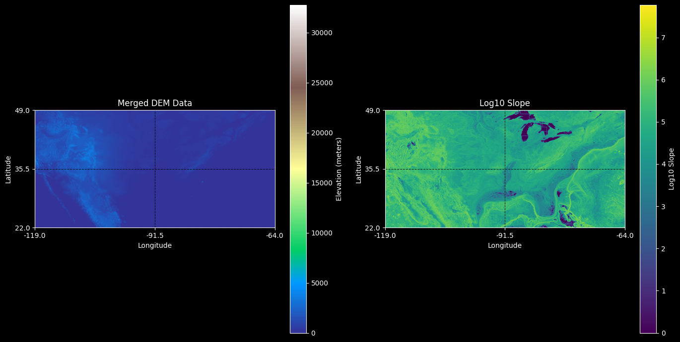
Show merged file as elevation heatmap
A beautiful thing about common Python libraries for geodata like rasterio is that they often have extremely sensible APIs for windowed or strided reading. Here’s a fast, IO efficient way to quickly create a plottable summary of the merged data by reading every 100-th pixel.
# Load the image and run imshow
if config.show_plots:
    with rasterio.open(merged_dem_path) as src:
        downsample_stride = 100
        dem_data = src.read(1,
        out_shape=(
            src.count,
            int(src.height / downsample_stride),
            int(src.width / downsample_stride)
        ),
        resampling=rasterio.enums.Resampling.nearest
     )


        # Calculate slope
        x, y = np.gradient(dem_data, src.res[0], src.res[1])
        slope = np.sqrt(x**2 + y**2)
        log_slope = np.log10(slope + 1)  # Adding 1 to avoid log(0)

        fig, axes = plt.subplots(1, 2, figsize=(14, 7))

        # Plot elevation
        im1 = axes[0].imshow(dem_data, cmap='terrain', extent=(bounds[0], bounds[2], bounds[1], bounds[3]), vmin=0)
        axes[0].set_title('Merged DEM Data')
        axes[0].set_xlabel('Longitude')
        axes[0].set_ylabel('Latitude')
        cbar1 = fig.colorbar(im1, ax=axes[0], orientation='vertical', label='Elevation (meters)')

        # Plot log10 slope
        im2 = axes[1].imshow(log_slope, cmap='viridis', extent=(bounds[0], bounds[2], bounds[1], bounds[3]))
        axes[1].set_title('Log10 Slope')
        axes[1].set_xlabel('Longitude')
        axes[1].set_ylabel('Latitude')
        cbar2 = fig.colorbar(im2, ax=axes[1], orientation='vertical', label='Log10 Slope')

        # Set the ticks to match the bounds
        for ax in axes:
            ax.set_xticks(np.linspace(bounds[0], bounds[2], num=3))
            ax.set_yticks(np.linspace(bounds[1], bounds[3], num=3))
            ax.xaxis.set_major_formatter(plt.FuncFormatter(lambda x, _: f'{x:.1f}'))
            ax.yaxis.set_major_formatter(plt.FuncFormatter(lambda y, _: f'{y:.1f}'))
            ax.grid(True, linestyle='--', alpha=0.8, color='k')

    plt.tight_layout()
    plt.show()
else:
    logging.info("Skipping display of merged DEM data. Set `show_plots` to True to display.")
9. Join elevation data with land cover data
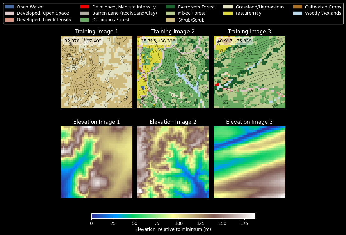
This is an especially delicate step. Just because you have done your best to make sure that the bounding box for the land cover extract and the elevation extract are the same, you may still get bad results due to minor errors in indexing or precision. At this point, some visual assessment of pixel-level accuracy of the coregistration of the two data layers is essential.
def extract_dem_images(gdf: gpd.GeoDataFrame, dem_src: rasterio.DatasetReader) -> np.ndarray[np.float32]:
    dem_images = []
    nodata_count = 0
    interpolate_count = 0

    for _, row in gdf.iterrows():

        window = rasterio.windows.from_bounds(*row.geometry.bounds, transform=dem_src.transform)

        dem_data = dem_src.read(1, window=window)

        is_nodata = dem_data == dem_src.nodata
        nodata_fraction = np.mean(is_nodata)
        dem_data = dem_data.astype(np.float32)

        # If the read failed, the shape will be empty so we raise an alarm
        # If any failure cases occur, we want the resulting DEM array to be all NaNs
        # and have all dims with nonzero size.
        if len(dem_data.shape) == 0:
            dem_data  = np.empty((config.image_size, config.image_size)) * np.nan
            logging.debug(f"Failed to read window for row {row} with window {window}")
            nodata_count += 1
        elif any([dim == 0 for dim in dem_data.shape]):
            dem_data = np.empty((config.image_size, config.image_size)) * np.nan
            logging.debug(f"Window read for row {row} with bbox {row.geometry.bounds} has a zero dimension with shape {dem_data.shape}")
            nodata_count += 1
        elif nodata_fraction > config.dem_nodata_threshold:
            dem_data *= np.nan
            nodata_count += 1
        elif np.any(is_nodata):
            # Interpolate NaN values using a spatially informed method
            mask = dem_data == dem_src.nodata
            dem_data = cv2.inpaint(dem_data, mask.astype(np.uint8), inpaintRadius=3, flags=cv2.INPAINT_TELEA)
            interpolate_count += 1

        # Resize using cv2 to the desired image size
        if not np.any(np.isnan(dem_data)):
            dem_data = cv2.resize(dem_data, (config.image_size, config.image_size), interpolation=cv2.INTER_LINEAR)

        dem_images.append(dem_data)

    logging.info(f"Number of images dropped due to nodata proportion exceeding threshold: {nodata_count} / {len(gdf)}")
    logging.info(f"Number of images with interpolation of missing values: {interpolate_count} / {len(gdf)}")
    return np.array(dem_images).astype(np.float32)

with rasterio.open(merged_dem_path) as dem_src:
    train_dem_images = extract_dem_images(train_gdf, dem_src)
    test_dem_images = extract_dem_images(test_gdf, dem_src)

# Offset all images to have a minimum of zero
train_dem_images -= train_dem_images.min(axis=(1, 2), keepdims=True)
test_dem_images -= test_dem_images.min(axis=(1, 2), keepdims=True)
/mnt/m2ssd/data/Dropbox/research/nlcd-inpaint/.venv/lib/python3.10/site-packages/numpy/core/fromnumeric.py:3504: RuntimeWarning: Mean of empty slice.
  return _methods._mean(a, axis=axis, dtype=dtype,
/mnt/m2ssd/data/Dropbox/research/nlcd-inpaint/.venv/lib/python3.10/site-packages/numpy/core/_methods.py:129: RuntimeWarning: invalid value encountered in scalar divide
  ret = ret.dtype.type(ret / rcount)
/tmp/ipykernel_348578/826475755.py:24: RuntimeWarning: invalid value encountered in multiply
  dem_data = np.empty((config.image_size, config.image_size)) * np.nan
[INFO] Number of images dropped due to nodata proportion exceeding threshold: 422 / 929184
[INFO] Number of images with interpolation of missing values: 0 / 929184
[INFO] Number of images dropped due to nodata proportion exceeding threshold: 142 / 227967
[INFO] Number of images with interpolation of missing values: 0 / 227967
Show DEM images
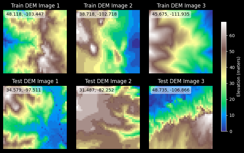
Let’s also make some pretty images of the elevation maps.
# Plot several train and test images using elevation colormap
if config.show_plots:
    n_images = 3
    fig, ax = plt.subplots(2, n_images, figsize=(8, 5))

    # Pick random sample of train and test images to show
    sampled_train_indices = np.random.choice(len(train_dem_images), n_images, replace=False)
    sampled_test_indices = np.random.choice(len(test_dem_images), n_images, replace=False)

    for i in range(n_images):
        for j, (images, gdf, title, sampled_indices) in enumerate(zip(
                [train_dem_images, test_dem_images],
                [train_gdf, test_gdf],
                ["Train DEM", "Test DEM"],
                [sampled_train_indices, sampled_test_indices])):

            im = ax[j, i].imshow(images[sampled_indices[i]], cmap='terrain')
            ax[j, i].set_title(f"{title} Image {i+1}")
            ax[j, i].axis('off')
            centroid = gdf.iloc[sampled_indices[i]].geometry.centroid
            ax[j, i].text(1.5, 3, f"{centroid.y:.3f}, {centroid.x:.3f}",color='black',
                          bbox=dict(facecolor='white', alpha=0.5, boxstyle='round,pad=0.3'))
            # Add gridlines and lat/long overlay
            ax[j, i].grid(True, linestyle='--', alpha=0.8, color='k')
            ax[j, i].set_xticks(np.linspace(0, config.image_size, num=3))
            ax[j, i].set_yticks(np.linspace(0, config.image_size, num=3))
            ax[j, i].set_xticklabels(np.linspace(centroid.x - config.image_size // 2, centroid.x + config.image_size // 2, num=3).round(2))
            ax[j, i].set_yticklabels(np.linspace(centroid.y - config.image_size // 2, centroid.y + config.image_size // 2, num=3).round(2))

    # Add a common colorbar on the right-hand side
    cbar_ax = fig.add_axes([1.0, 0.15, 0.02, 0.7])
    fig.colorbar(im, cax=cbar_ax, orientation='vertical', label='Elevation (meters)')

    plt.tight_layout(rect=[0.1, 0, 1, 1])
    plt.show()
else:
    logging.info("Skipping DEM image visualization; set show_plots to True to display images.")
# Create visualization of NLCD and DEM data
n_images = 3
seen_classes = set()
if config.show_plots:
    fig, axes = plt.subplots(2, n_images, figsize=(n_images*2.5, 8))

    # Pick random sample of train images to show

    sampled_indices = np.random.choice(len(train_images), n_images, replace=False)

    # Plot first n_images from training set
    for i, sample_idx in enumerate(sampled_indices):

        # Get DEM data for this image
        dem = train_dem_images[sample_idx]
        dem_min = dem.min()
        dem_relative = dem - dem_min

        # Calculate contours (relative to minimum elevation)
        levels = np.linspace(0, dem_relative.max(), 10)

        # Plot NLCD with contours
        axes[0, i].imshow(lut[train_images[sample_idx]])
        cs = axes[0, i].contour(dem_relative, levels=levels, colors='k', alpha=0.7, linewidths=0.5)
        axes[0, i].clabel(cs, inline=True, fontsize=8, fmt='%.0f')
        axes[0, i].set_title(f'Training Image {i+1}')
        axes[0, i].axis('off')

        # Add lat/lon labels to image
        centroid = train_gdf.iloc[sample_idx].geometry.centroid
        axes[0, i].text(1.5, 3, f"{centroid.y:.3f}, {centroid.x:.3f}", color='black',
                        bbox=dict(facecolor='white', alpha=0.5, boxstyle='round,pad=0.3'))
        axes[0, i].grid(True, linestyle='--', alpha=0.8, color='k')

        # Plot DEM
        im = axes[1, i].imshow(dem, cmap='terrain')
        axes[1, i].set_title(f'Elevation Image {i+1}')
        axes[1, i].axis('off')
        seen_classes.update(np.unique(train_images[sample_idx]))

    # Add colorbar for elevation below the subplots
    cbar_ax = fig.add_axes([0.15, 0.12, 0.7, 0.02])
    fig.colorbar(im, cax=cbar_ax, orientation='horizontal', label='Elevation, relative to minimum (m)')

    # Add legend for NLCD classes above the subplots
    legend_handles = [mpatches.Patch(color=classes_df.loc[idx, "RGB"],
                                     label=classes_df.loc[idx, "name"])
                      for idx in seen_classes]
    fig.legend(handles=legend_handles, loc='upper center',
               bbox_to_anchor=(0.5, 0.99), ncol=5)

    plt.tight_layout(rect=[0, 0.1, 1, 0.95])
    plt.show()
else:
    logging.info("Skipping visualization of NLCD and DEM data; set show_plots=True to enable.")
10. Concatenate data and save to disk
Now that we’ve done all the hard work, let’s finally save our data to disk. It is popular to use data packaging formats like hdf5, xarray, and so on. These can be useful, but remember - you need to do everything you can to make it easier for your future self to jump back into the work with short notice. Just be simple and sensible by saving an array in shape N, C, H, W. You’ll know which channel is which just by looking at the elements.
is_image_bad_train = np.any(np.isnan(train_dem_images), axis=(1, 2))
is_image_kept_train = ~is_image_bad_train

train_images_final = train_images[is_image_kept_train]
train_dem_images_final = train_dem_images[is_image_kept_train]
train_gdf_final = train_gdf[is_image_kept_train]
logging.info(f"Removed {is_image_bad_train.sum()} images with missing DEM data from training set.")

is_image_bad_test = np.any(np.isnan(test_dem_images), axis=(1, 2))
is_image_kept_test = ~is_image_bad_test
test_images_final = test_images[is_image_kept_test]
test_dem_images_final = test_dem_images[is_image_kept_test]
test_gdf_final = test_gdf[is_image_kept_test]
logging.info(f"Removed {is_image_bad_test.sum()} images with missing DEM data from test set.")

# Take arrays of shape (N, H, W) and stack them along the channel axis
# which needs to be created for both data sets
train_combined = np.stack([train_images_final, train_dem_images_final], axis=1)
np.save(config.output_path_train, train_combined)
train_file_size = os.path.getsize(config.output_path_train)
logging.info(f"Training Numpy array with shape {train_combined.shape} saved to {config.output_path_train} (Size: {train_file_size / (1024 * 1024):.2f} MB)")

test_combined = np.stack([test_images_final, test_dem_images_final], axis=1)
np.save(config.output_path_test, test_combined)
test_file_size = os.path.getsize(config.output_path_test)
logging.info(f"Test data Numpy array with shape {test_combined.shape} saved to {config.output_path_test} (Size: {test_file_size / (1024 * 1024):.2f} MB)")

train_gdf_final.to_file(config.output_path_train.with_suffix('.gpkg'), driver='GPKG')
train_gpkg_size = os.path.getsize(config.output_path_train.with_suffix('.gpkg'))
logging.info(f"Training sample location GeoDataFrame saved to {config.output_path_train.with_suffix('.gpkg')} (Size: {train_gpkg_size / (1024 * 1024):.2f} MB)")

test_gdf_final.to_file(config.output_path_test.with_suffix('.gpkg'), driver='GPKG')
test_gpkg_size = os.path.getsize(config.output_path_test.with_suffix('.gpkg'))
logging.info(f"Test sample location GeoDataFrame saved to {config.output_path_test.with_suffix('.gpkg')} (Size: {test_gpkg_size / (1024 * 1024):.2f} MB)")
[INFO] Removed 422 images with missing DEM data from training set.
[INFO] Removed 142 images with missing DEM data from test set.
[INFO] Training Numpy array with shape (928762, 2, 40, 40) saved to /mnt/m2ssd/data/Dropbox/research/nlcd-inpaint/generative-land-cover/data/train.npy (Size: 22674.85 MB)
[INFO] Test data Numpy array with shape (227825, 2, 40, 40) saved to /mnt/m2ssd/data/Dropbox/research/nlcd-inpaint/generative-land-cover/data/test.npy (Size: 5562.13 MB)
[INFO] Training sample location GeoDataFrame saved to /mnt/m2ssd/data/Dropbox/research/nlcd-inpaint/generative-land-cover/data/train.gpkg (Size: 185.46 MB)
[INFO] Test sample location GeoDataFrame saved to /mnt/m2ssd/data/Dropbox/research/nlcd-inpaint/generative-land-cover/data/test.gpkg (Size: 45.86 MB)
11. Make an animation
Cleaning and processing data is pure drudgery and I am sorry that you have to do it. Hopefully in ten years we will have a better solution than doing it ourselves.
The best way you can make it palatable is to make something pretty. Make something that gives you joy when you look at it, because joy is rare here. Through much trial and error, I’ve found that (besides high-impact publications), what makes colleagues the happiest is a nice animation that gives them something to think about.
Always try to give your peers some eye candy.
import numpy as np
import matplotlib.pyplot as plt
import cv2
from matplotlib.animation import FuncAnimation
import matplotlib as mpl
from concurrent.futures import ThreadPoolExecutor
from functools import partial

class TerrainAnimator:
    def __init__(self, train_images, train_dem_images, lut, n_rows=4, n_cols=8):
        self.train_images = train_images
        self.train_dem_images = train_dem_images
        self.lut = lut
        self.n_rows = n_rows
        self.n_cols = n_cols
        self.exaggeration = 1

        # Pre-calculate mesh grid
        self.h, self.w = train_images[0].shape
        x = np.arange(self.w)
        y = np.arange(self.h)
        self.X, self.Y = np.meshgrid(x, y)

        # Initialize figure
        self.setup_figure()

    def setup_figure(self):
        plt.rcParams['figure.dpi'] = 150
        self.fig, self.axes = plt.subplots(
            self.n_rows,
            self.n_cols,
            figsize=(self.n_cols*1.4, self.n_rows*1.6),  # Reduced figure size
            subplot_kw={'projection': '3d'},
            constrained_layout=True  # Use constrained layout
        )
        self.fig.set_facecolor('black')
        self.fig.patch.set_alpha(1.0)
        # Reduce margins
        plt.subplots_adjust(left=0.02, right=0.98, bottom=0.02, top=0.98)

        # Select random indices once
        self.indices = np.random.choice(
            len(self.train_images),
            self.n_rows * self.n_cols,
            replace=False
        )

    def process_elevation(self, elevation):
        """Pre-process elevation data with Gaussian smoothing"""
        return cv2.GaussianBlur(elevation, (5, 5), 0)

    def create_surface(self, ax, idx):
        """Create a single surface plot"""
        land_cover = self.train_images[idx]
        elevation = self.process_elevation(self.train_dem_images[idx])

        surf = ax.plot_surface(
            self.X, self.Y,
            elevation * self.exaggeration,
            facecolors=self.lut[land_cover],
            shade=False,
            antialiased=False,
            rstride=1,
            cstride=1
        )

        # Configure view
        ax.view_init(elev=30, azim=45)
        ax.set_box_aspect([1, 1, 0.5])

        # Remove unnecessary elements
        ax.set_xticks([])
        ax.set_yticks([])
        ax.set_zticks([])
        ax.grid(False)
        ax.axis('off')

        ele_max = elevation.max()

        if ele_max < 100:
            zlim = 150
        elif ele_max < 200:
            zlim = 250
        else:
            zlim = max(300, ele_max * 3)

        ax.set_zlim(0, zlim)

        return surf

    def setup_plots(self):
        """Initialize all surface plots in parallel"""
        with ThreadPoolExecutor() as executor:
            self.surfaces = list(executor.map(
                lambda args: self.create_surface(*args),
                zip(self.axes.flatten(), self.indices)
            ))

        plt.subplots_adjust(hspace=-0.6, wspace=-0.2)  # Increased overlap between subplots

    def update(self, frame):
        """Animation update function"""
        for ax in self.axes.flatten():
            ax.view_init(elev=30, azim=frame)
        return self.surfaces

    def create_animation(self, frames=360, fps=30):
        """Create and save the animation"""
        self.setup_plots()

        anim = FuncAnimation(
            self.fig,
            self.update,
            frames=frames,
            interval=1000/fps,
            blit=True
        )

        # Save with optimized settings
        anim.save(
            'terrain_rotation.gif',
            writer='pillow',
            fps=fps,
            savefig_kwargs={'facecolor': 'black'},
            progress_callback=lambda i, n: print(f'Saving frame {i}/{n}', end='\r')
        )
        plt.close()


train_images_final = np.load(config.output_path_train)
anim_images_lc = train_images_final[:, 0].astype(int)
anim_images_dem = train_images_final[:, 1]

# Usage
animator = TerrainAnimator(anim_images_lc, anim_images_dem, lut)
animator.create_animation()
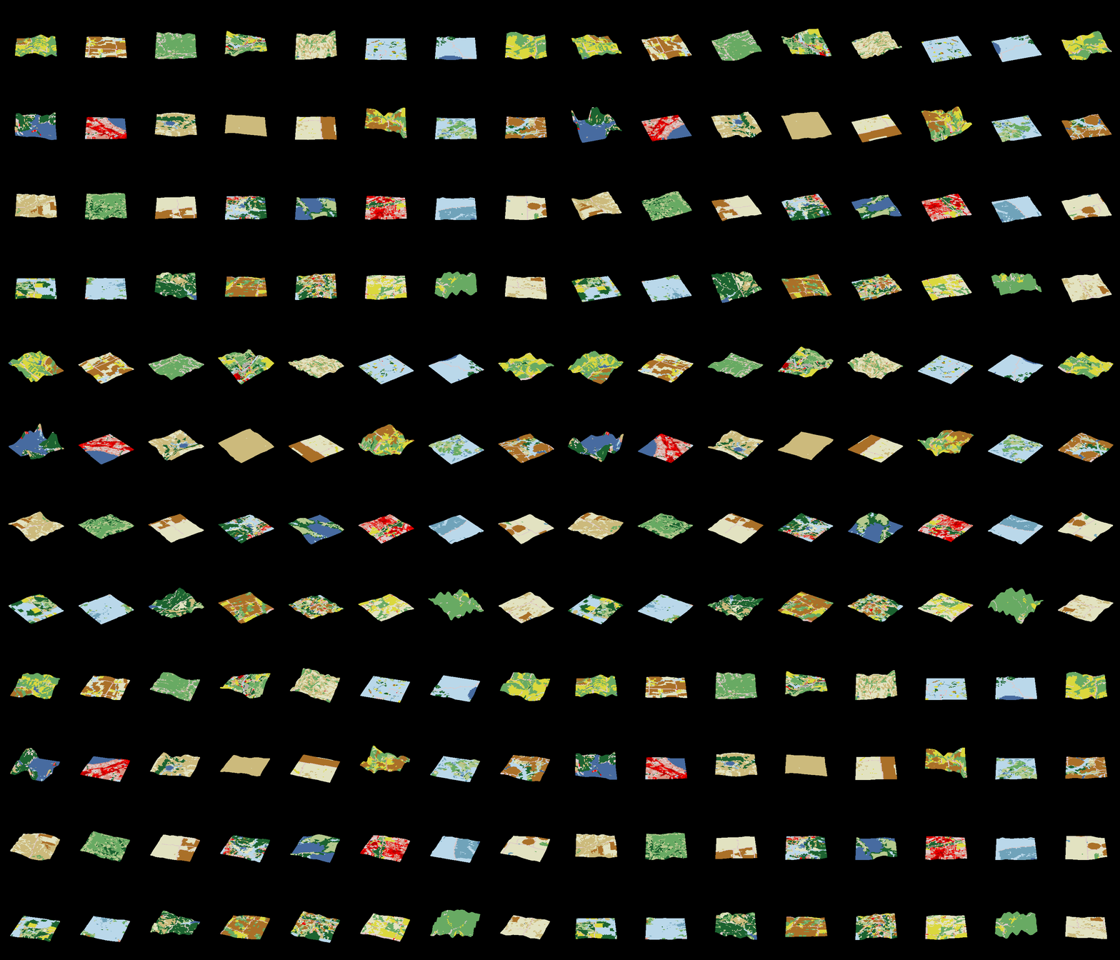
With this code, we get some nice visualizations of our data samples, rotating and shown in 3D!
Epilogue: optimization
Once you have your code running for a small test dataset, you can go back and try to figure out how to improve it. Runtime is important, but the bigger issue (in my experience) is space in memory as you can always just let a job run longer. You can’t easily give your computer more working memory on the spot. For this, I strongly recommend a command like %whos to get a dataframe of variables and their size in memory. Sort it if you like, but focus on the ones with the biggest footprint.
%whos
Variable                     Type              Data/Info
--------------------------------------------------------
...                          ...               ...
x                            ndarray           972x1980: 1924560 elems, type `float64`, 15396480 bytes (14.6832275390625 Mb)
x_edges                      ndarray           51: 51 elems, type `float64`, 408 bytes
y                            ndarray           972x1980: 1924560 elems, type `float64`, 15396480 bytes (14.6832275390625 Mb)
y_edges                      ndarray           51: 51 elems, type `float64`, 408 bytes
Enjoy Reading This Article?
Here are some more articles you might like to read next: