Modeling data with correlated errors across a directed graph

Data for objects which can be linked together with a graph are common in fields like epidemiology and sociology. A simple way to model this kind of data is with a linear mixed model with a random effect with some network structure, or an error term which is correlated. The former is appropriate when you have multiple observations for each node in your graph while the latter is applicable when there is usually just one data point for each node.

PyMC has functionality for these kinds of models assuming an undirected graph. This makes sense if it’s not clear which way the causality goes. For example, if the number of infected people in city \(A\) is correlated with the same quantity in city \(G\) because there is a road from \(A\) to \(G\), then the correlation could be due to people traveling from \(A\) to \(G\), from \(G\) to \(A\), or both processes simultaneously. This is a great opportunity to use a Gaussian Markov random field, synonomous with conditional autoregression.

Many real-world networks are actually directed graphs, however. An example of this type is a river network. Water flows in one direction, and events like floods or pollutant spills which occur downstream will generally not have an effect on the upstream segments of the network.

In the case where we have a directed graph, we can use some tricks from linear algebra to account for this network-based correlation to help produce more accurate estimates of regression coefficients and better predictive performance on new data. In this post, we’ll use some basic matrix facts and identities to implement a highly scalable and effective linear mixed model for network data assuming an underlying directed acyclic graph (DAG). To learn more about these terms and concepts, I highly recommend selected chapters from Statistical Rethinking and Probabilistic Graphical Models.

import arviz as az
import numpy as np
import pymc as pm
import pytensor.tensor as pt
import pytensor.sparse as sparse
import scipy as sp
import seaborn as sns
import xarray as xr

from matplotlib import pyplot as plt
from matplotlib.lines import Line2D
from numpy.random import default_rng
from xarray_einstats import linalg
from xarray_einstats.stats import XrContinuousRV

print(f"Running on PyMC v{pm.__version__}")
%config InlineBackend.figure_format = 'retina'
az.style.use("arviz-darkgrid")

np.set_printoptions(precision=3, suppress=True)
RANDOM_SEED = 8271991
rng = default_rng(RANDOM_SEED)

Model structure

To illustrate why we should account for any underlying network structure in our dataset, let’s start with an example using synthetic data. We’ll assume the following probabilistic model for \(N\) data points for the rest of the notebook:

We’ll use \(P = 2\) in this example, though the role of the linear predictor \(X \beta\) is not important. \(\mathbf{y}\) is a vector of observations with correlated errors; the structure of this correlation is encoded in the elements of \(\Sigma\), an \(N\times N\) covariance matrix.

Another assumption we will make is that the index \(i \in \{1,...,N\}\) maps individual data points to locations on a directed acyclic graph \(G\). \(G\) can be represented as a binary, asymmetric matrix. Gaussian DAG models (sometimes also described as continuous Bayesian networks) have the nice feature that their underlying correlation structure can be described in terms of an inverse-covariance matrix \(\Lambda\), also referred to as the precision matrix.

Assuming that the index \(i\) respects the topological order of the graph \(G\), the zeros of the precision matrix tell us which elements are conditionally independent. Put differently, if \(\lambda_{ij}\) is zero, then \(\epsilon_i\) and \(\epsilon_j\) are independent given all other elements of \(\mathbf{\epsilon}\)

To understand this matrix, note that the diagonal elements \(\sigma_1, ...\) control the scale of the random variables while the off-diagonal elements control the correlation between \(y_i\) and \(y_j\). This matrix is equivalent (under Gaussian conditions) to the following graphical diagram:

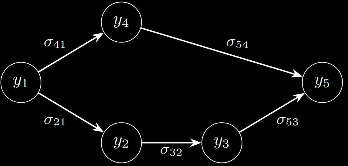
We can actually simulate data with this correlation structure easily given \(\Lambda\) as shown in the next section. This graph also has an interpretation via the LDL factorization of \(\Lambda\). Noting that \(\Lambda\) is positive semi-definite, it can be written as:

\(\Lambda = (I-\mathcal{G})^T\Omega(I-\mathcal{G})\) where \(I\) denotes the identity matrix, \(\mathcal{G}\) is a triangular matrix, and \(\Omega\) is a diagonal matrix containing the scalar precision values on its diagonal. While the elements of \(\mathcal{G}\) can be distinct, having one parameter for every nonzero value of \(\mathcal{G}\) is unnecessary as that implies a unique precision parameter for every edge in the graph \(G\). Instead, we typically work with a parameterization of \(\mathcal{G}\) in terms of a scalar parameter \(\gamma\) and the binary matrix \(G\) with \(\mathcal{G}= \gamma G\). Our interpretation of \(\mathcal{G}\) is quite interesting - it gives a construction for draws of \(\epsilon_j\) via regression on elements occurring earlier in the topological order:

One may interpret this as saying that the error term for node \(j\) can be written as a linear combination of error terms from nodes that precede it in the topological ordering of the graph, plus an independent noise term \(\nu_j\). The coefficient \(b_{ji}\) represents the strength of the relationship between nodes \(i\) and \(j\), and is nonzero only when there is a directed edge from node \(i\) to node \(j\) in the graph.

Simulated data generation

To fully illustrate how to use this model, we’ll begin by creating a dataset reflective of a regression with DAG-structured error terms.

n       = 29 # Number of samples, also dimension of the covariance matrix
n_edges = n * 2

p = 2  # Number of predictors

beta_true = np.asarray([-0.5, 0.5])

# In the directed graph, the coefficients for each element of eps in terms of the
# previous elements with edges in the graph
rho = 1.0

x = rng.normal(size=(n, p))
eps_raw = rng.normal(size=(n))

def sample_sparse_dag(n: int, n_edges: int) -> sp.sparse.lil_matrix:
    '''
    Sample `n_pairs` pairs of edges from a directed graph with `n` nodes.
    Edges are not allowed to point to themselves. Assumes topological ordering
    of the nodes.
    '''
    G = sp.sparse.lil_matrix((n, n), dtype=int)

    # First, make sure that each node has at least one child
    # except for the last node
    for i in range(n-1):
        j = rng.integers(i+1, n)
        G[i, j] = True

    for i in range(n_edges - n):
        # Sample a pair of nodes
        # such that i < j
        i = rng.integers(0, n-1)
        j = rng.integers(i+1, n)

        if i == j or G[i, j]:
            continue
        G[i, j] = True

    return G.tocsr()

# parent idx is i, child idx is j
G = sample_sparse_dag(n, n_edges)
#G = np.zeros((n, n), dtype=int)
G = sp.sparse.csr_matrix(G)

eps = np.zeros(n)

for j in range(n):
    eps[j] = eps_raw[j]
    for i in range(n):
        if G[i, j]:
            eps[j] += rho * eps[i]


y = x @ beta_true + eps

If we visualize the resulting DAG matrix as a heatmap, we can see the sparse, triangular structure as desired.

Next, we’ll fit two models. The first model naively assumes that elements of \(\mathbf{y}\) are conditionally independent given \(X\beta\). The second model explicitly accounts for the correlated graph structure. In practice, we will often know whether the elements \(i,j\) share an edge, but we won’t know exactly how strong the correlation between them should be.

with pm.Model() as naive_model:
    β = pm.Normal("β", 0, 5, shape=p)
    error_sigma = pm.HalfNormal("error_sigma", 1)
    
    _ = pm.Normal("y",
        mu=pt.dot(x, β),
        sigma=error_sigma,
        observed=y,
    )

with pm.Model() as graph_model:
    β = pm.Normal("β", 0, 5, shape=p)

    ω = pm.HalfNormal("ω", 1) # Controls uncorrelated variance
    γ = pm.HalfNormal("γ", 1) # Controls correlation between nodes in graph

    G_pt = pm.math.constant(np.asarray(G.astype(float).todense()))
    Ω = pt.diag(pt.ones(n)) * ω
    I = pt.eye(n)
    
    IminusG = I -  γ * G_pt
    tau = ω * IminusG @ IminusG.T # Precision matrix

    _ = pm.MvNormal("y",
        mu=pt.dot(x, β),
        tau=tau,
        observed=y,
    )

with naive_model:
    trace_naive = pm.sample()

with graph_model:
    trace_graph = pm.sample()

fig, axs = plt.subplots(2, 2, figsize=(9, 7), sharex="col")

az.plot_posterior(trace_naive, var_names=["β"], coords={"β_dim_0": 0}, ax=axs[0, 0], color="C0")
axs[0, 0].axvline(beta_true[0], color="k", linestyle="--")
axs[0, 0].set_title(f"Naive Model - β₀ (True value: {beta_true[0]:.2f})")

az.plot_posterior(trace_naive, var_names=["β"], coords={"β_dim_0": 1}, ax=axs[0, 1], color="C0")
axs[0, 1].axvline(beta_true[1], color="k", linestyle="--")
axs[0, 1].set_title(f"Naive Model - β₁ (True value: {beta_true[1]:.2f})")

az.plot_posterior(trace_graph, var_names=["β"], coords={"β_dim_0": 0}, ax=axs[1, 0], color="C1")
axs[1, 0].axvline(beta_true[0], color="k", linestyle="--")
axs[1, 0].set_title(f"Graph Model - β₀ (True value: {beta_true[0]:.2f})")

az.plot_posterior(trace_graph, var_names=["β"], coords={"β_dim_0": 1}, ax=axs[1, 1], color="C1")
axs[1, 1].axvline(beta_true[1], color="k", linestyle="--", label="True value of β₁")
axs[1, 1].set_title(f"Graph Model - β₁ (True value: {beta_true[1]:.2f})")

plt.tight_layout()

Using the MvNormal likelihood took longer, but the advantages are clear: after accounting for the correlated errors, our coefficient estimates are much better in terms of HDI width as well as distance between the posterior mean and the true value used to produce the dataset.

Unfortunately, using the MvNormal likelihood in this example incurs a \(\mathcal{O}(N^3)\) computation cost from applying the Cholesky decomposition to \(\Sigma\) in order to compute \(\log p(\mathbf{y} \mid \mathbf{\mu}, \Sigma )\).

Having set the basic context for modeling, let’s discuss some concrete computational considerations for conducting inference more efficiently:

• First, by assuming which elements of \(\mathbf{\epsilon}\) depend on each other in a DAG-structured manner, we can model the covariance of \(\mathbf{\epsilon}\) in terms of a lower-triangular factorized form of \(\Lambda\) and thus \(\Sigma\).
• The two main sources of computational cost for modeling with a multivariate normal likelihood are (1) the determinant of the covariance matrix, \(\det(\Sigma)\), and (2) the calculation of the inner product \(\mathbf{\epsilon}^T \Lambda \mathbf{\epsilon}\)

We will use the structural assumptions of our model to make these operations cheaper. Beginning with (1), our assumptions for \(\Lambda\) let us write the following by using some basic matrix identities:

This gives us an \(\mathcal{O}(N)\) formula for \(\det(\Sigma)\) which normally requires \(\mathcal{O}(N^3)\) computation with relaxed assumptions. We are fortunate here that \(\det(I-\gamma G) = 1\) as the determinant of a triangular matrix is given by the product of its diagonals; since \(G\) has no diagonal elements and \(I\) is the identity matrix, this product is equal to 1.

For item (2) from above, we can rewrite \(\mathbf{\epsilon}^T \Lambda \mathbf{\epsilon}\) as \(\mathbf{u} = \mathbf{\epsilon}^T (I - \gamma G)^T \Omega^{1/2}\) such that \(\mathbf{\epsilon}^T \Lambda \mathbf{\epsilon} = \mathbf{u}^T\mathbf{u}\). Since \(\Omega\) is diagonal, \(\Omega^{1/2}\) is just the elementwise square root of \(\Omega\). Then, since \(G\) is sparse, the dot product \(\mathbf{\epsilon}^T(I-\gamma G)\) will also be relatively cheap.

We can also make a few more simplifications. Until now, we assumed that we would use \(n\) distinct values of \(\omega_{ii}\) for modeling. In practice, this means a separate precision parameter for each observation which is unnecessary. We’ll instead work with a single global precision parameter \(\omega\) so that \(\Omega = \omega I\), letting us simplify a few more operations.

We can also simplify this model a bit:

This approach is capable of scaling out to a very large number of dimensions, in theory. Below is a work-in-progress implementation to try to do this. Unfortunately, there are some PyTensor issues that arise when trying to sample with this.

I = sp.sparse.eye(n, format="csr", dtype=float)
n = len(y)
with pm.Model() as sparse_graph_model:
    β = pm.Normal("β", 0, 5, shape=p)
    μ = pt.dot(x, β)
    ε = pm.math.constant(y) - μ

    ω = pm.HalfNormal('ω', 1) # controls the diagonal entries of the precision matrix
    γ = pm.HalfNormal("γ", 1) # controls the off-diagonal entries of the precision matrix

    G_pt = sparse.as_sparse_or_tensor_variable(G.astype(float))
    I_pt = sparse.as_sparse_or_tensor_variable(I)

    # Make ε be shape (n,1)
    ε_col = ε[:, None]
    Gε = sparse.structured_dot(G_pt, ε_col)
    γGε = γ * Gε
    print(f"Shape of Gε: {Gε.shape.eval()}")
    print(f"Shape of γGε: {γGε.shape.eval()}")

    resid = ε - γGε.squeeze()

    # For quadratic form εᵀ(I-γG)ᵀΩ(I-γG)ε
    # This is equivalent to ω * (ε - γGε)(ε - γGε)ᵀ
    quadratic_form = ω * pt.sum(resid**2)
        
    logdet = n * pt.log(ω)
    logp =  -0.5 * (n * pt.log(2 * np.pi) + logdet + quadratic_form )
    pm.Potential('likelihood', logp)

    trace_sparse_graph = pm.sample()

If we look at the two traces, they are very different. I’m not sure what’s causing the discrepancy. If you do know, please tell me!

az.summary(trace_graph)
az.summary(trace_sparse_graph)