Spline regression in PyMC3

Linear regression is a useful tool but is limited in the expressivity of functional relations which it can capture. Once we move to nonlinear regression, we have tons of options and a hard question to answer - how do we specify our model?

One of the most popular options is to use a piecewise polynomial representation. That is, we take multiple polynomials and stitch them together at break or control points. If we intelligently choose the right basis for this function, then are also guaranteed that the polynomials (and their derivatives) will agree at the control points. That’s the underlying idea behind splines. There is a convenient basis for a spline function in terms of other splines which is generally referred to as a basis-spline or B-spline. In this notebook, I’ll go over a simple example of using a B-spline component in a regression model. Most of the Theano code is cribbed directly from the Github account of the Kundaje lab at Stanford and appears to have been written by a researcher named Nathan Boley. I’d like to share it here (with modification) so that we can see how to use a flexible function approximation scheme like a B-spline to loosen our modeling assumptions.

If you’re new to modeling with B-splines, I suggest reading the Wikipedia page or this page from Ching-Kuang Shene at Michigan Tech

Imports

As usual, the main packages we’ll use are PyMC3 and Theano. Numpy is used only to help generate some synthetic data. Matplotlib is used to visualize the results.

import matplotlib.pyplot as plt
import numpy as np
import theano
import theano.tensor as tt
import pymc3 as pm
%matplotlib inline

Theano can be fairly picky with its settings. These directives specify to always use a more-expressive data type and to bypass test value checking.

theano.config.floatX = 'float64'
theano.config.compute_test_value = 'ignore'

Theano implementation of B-splines

In order to use PyMC3 to maximum effect (i.e. with NUTS using the model gradients for MCMC), we need to make sure that the entire spline generative process is specified in Theano. Therefore, we need to write Theano functions which take the spline breakpoints and coefficients to create a spline curve \(f(x)\). This spline curve will be represented by a function which can be evaluated at various values of \(x\) over some domain \([u_0,u_m]\).

The code flow largely matches the recursive de Boor formula - this algorithm begins by specifying zero-order polynomials (aka step functions), specifying the first-order polynomials in terms of the zero-th, and so on and so forth. It’s an elegant scheme, even if you have to stare at it for awhile to follow what it’s doing.

This first function simply creates a list of Theano tensors. Each tensor represents a step function over a different part of the domain. The switch statements are used to create the step functions. The array breaks needs to contain all the interior control points in the correct order, as well as the left endpoint and the right endpoint at the beginning and end of the array, respectively. The second argument, x, should specify the domain of the spline. For example, if we want the spline to run over the interval \([0,5]\), then we should set x to something like np.linspace(0,5).

def build_B_spline_deg_zero_degree_basis_fns(breaks, x):
    """Build B spline 0 order basis coefficients with knots at 'breaks'. 
    N_{i,0}(x) = { 1 if u_i <= x < u_{i+1}, 0 otherwise }
    """
    expr = []
    expr.append(tt.switch(x<breaks[1], 1, 0))
    for i in range(1, len(breaks)-2):
        l_break = breaks[i]
        u_break = breaks[i+1]
        expr.append(
            tt.switch((x>=l_break)&(x<u_break), 1, 0) )
    expr.append( tt.switch(x>=breaks[-2], 1, 0) )
    return expr

Once this list of zero-order basis functions is created, we’ll use it to define the higher order basis functions. The next function does just that; it doesn’t operate on any specific level or degree and can be used over and over again for a higher degree spline. This is exactly the recursion formula given on the Wikipedia page for the de Boor algorithm.

def build_B_spline_higher_degree_basis_fns(
        breaks, prev_degree_coefs, degree, x):
    """Build the higer order B spline basis coefficients
    N_{i,p}(x) = ((x-u_i)/(u_{i+p}-u_i))N_{i,p-1}(x) \
               + ((u_{i+p+1}-x)/(u_{i+p+1}-u_{i+1}))N_{i+1,p-1}(x)
    """
    assert degree > 0
    coefs = []
    for i in range(len(prev_degree_coefs)-1):
        alpha1 = (x-breaks[i])/(breaks[i+degree]-breaks[i]+1e-12)
        alpha2 = (breaks[i+degree+1]-x)/(breaks[i+degree+1]-breaks[i+1]+1e-12)
        coef = alpha1*prev_degree_coefs[i] + alpha2*prev_degree_coefs[i+1]
        coefs.append(coef)
    return coefs

So, to recap, we’ve defined a function to get us started with the first level of spline basis functions and then another to recursively define the rest of them. Finally, we need a loop to go ahead and apply the recursive function until the maximum degree is reached.

def build_B_spline_basis_fns(breaks, max_degree, x):
    curr_basis_coefs = build_B_spline_deg_zero_degree_basis_fns(breaks, x)
    for degree in range(1, max_degree+1):
        curr_basis_coefs = build_B_spline_higher_degree_basis_fns(
            breaks, curr_basis_coefs, degree, x)
    return curr_basis_coefs

Note that this only gives us our basis functions. We still have to express the desired spline function in terms of this basis. Fortunately, that’s straightforward because any spline can be represented with this basis. In spline_fn_expr, the variable intercepts designates how much of each basis function is used in a linear combination. Remember that we are not manipulating explicit numerical variables with a known value - we are doing arithmetic with Theano tensors and building a computational graph.

def spline_fn_expr(breaks, intercepts, degree, x):
    basis_fns = build_B_spline_basis_fns(breaks, degree, x)
    spline = 0
    for i, basis in enumerate(basis_fns):
        spline += intercepts[i]*basis
    return spline

None of this code can be used to directly generate numerical values until we compile the computational graph using theano.function. In the function below, there are some manipulations of the breaks array to pad with extra values. I’m not sure of what’s going on there.

def compile_spline(data,n_bins,degree,intercepts):
    breaks = np.histogram(data, n_bins)[1][1:-1]
    for i in range(degree+1):
        breaks = np.insert(breaks, 0, data.min()-1e-6)
        breaks = np.append(breaks, data.max()+1e-6)
    xs = tt.vector(dtype=theano.config.floatX)
    f = theano.function([intercepts, xs],spline_fn_expr(breaks, intercepts, degree, xs))
    return f

Let’s go ahead and try to generate some synthetic data.

Generating synthetic data from a spline

In this example, we’ll assume the spline has support over \([-4,4]\) and has a degree of 4. This means that each piecewise polynomial is going to be cubic.

domain = np.linspace(-4,4,100)
n_bins = 4
degree = 4
coefficients = tt.vector(dtype=theano.config.floatX)
spline = compile_spline(domain,n_bins,degree,coefficients)

We’ll also work with 20 randomly generated data points. The number of coefficients needed with four bins and a degree of 4 is \(4+4+1=9\) so our coefficient vector is 9 long.

x = np.asarray([-3.69,  1.60, -2.05, -1.63, -3.07,
       -1.06,  3.64, -1.61, -2.58, -3.57,
       -1.55, -1.93, -3.94,  3.51, -0.17,
       -3.92,  0.52,  3.06 ,  3.40, -0.21])
true_coef = np.asarray([ 0.82, -0.34,  1.75, -0.78,  0.25,
       -0.76,  0.59,  1.13 ,  1.32])

Now that the spline generating function is compiled and we have some input data, we can generate some spline values and add some noise to them.

true_mean   = spline(true_coef,domain)
y_noiseless = spline(true_coef,x)

y_noisy = y_noiseless + np.random.randn(x.shape[0])*0.2

plt.scatter(x,y_noisy,label = 'Noisy realizations of \nspline-valued process',color='k')
plt.plot(domain,true_mean,color='k',label = 'True function value')
plt.legend(loc = 'lower left')
plt.xlabel('x')
plt.ylabel('f(x)')
plt.savefig('noisy_spline.png',dpi = 400)

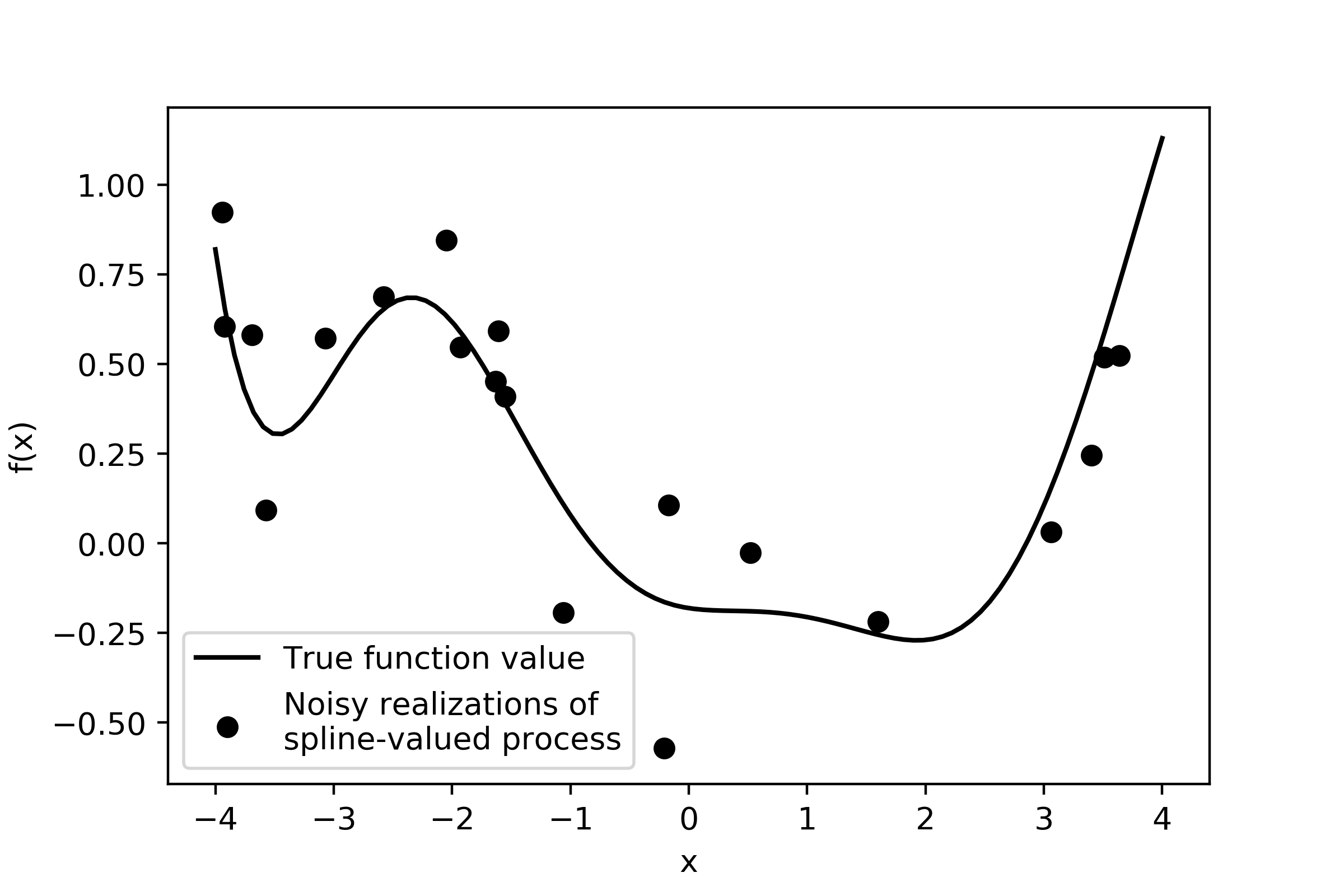
The noise standard deviation is only 0.2, so the noisy data points won’t fall far from the spline curve. The next section shows how we’d estimate the spline parameters using PyMC3.

Estimate spline parameters

As we attempt to recover the original spline curve, we’ll assume that we know the appropriate number of breakpoints and the polynomial degree. This is a major assumption - we probably won’t know these things in practice.

n_bins = 4
degree = 4
num_coef = n_bins + degree + 1 # Restraint that must be obeyed by parameter sets of B-splines
domain   = np.linspace(-4,4,100)

Next, there’s a sort of hack to make sure the breaks vector’s behavior matches up with what the earlier spline function does.

breaks = np.histogram(domain, n_bins)[1][1:-1]
for i in range(degree+1):
    breaks = np.insert(breaks, 0, domain.min()-1e-6)
    breaks = np.append(breaks, domain.max()+1e-6)

Finally, we can start writing down the statistical model. We’ll put a flat (i.e. uninformative) prior on the spline coefficients. We also need to cast our input data x-coordinate into a Theano tensor type. Normally PyMC3 handles this casting behind the scenes, but since we are writing our own custom variable type, we have to do it ourselves.

with pm.Model() as model:   
    coef   = pm.Flat('coef',shape = num_coef,testval = np.zeros(num_coef))
    x_as_tensor = tt.as_tensor(x)
    s = spline_fn_expr(breaks, coef, degree, x_as_tensor)

Finally, the rest of this model looks like a standard regression with unknown variance. I put a positive Cauchy prior on the error standard deviation and use NUTS to estimate the parameters.

with model:
    sigma  = pm.HalfCauchy('sigma',beta=1.0)
    y_hat  = pm.Deterministic('y_hat',s)
    y      = pm.Normal('y',mu = y_hat,sd = sigma,observed = y_noisy)
    trace  = pm.sample(chains=1)

Auto-assigning NUTS sampler...
Initializing NUTS using jitter+adapt_diag...
Sequential sampling (1 chains in 1 job)
NUTS: [sigma_log__, coef]
100%|██████████| 1000/1000 [01:57<00:00,  8.52it/s]
The chain reached the maximum tree depth. Increase max_treedepth, increase target_accept or reparameterize.
Only one chain was sampled, this makes it impossible to run some convergence checks

Let’s see how well we did at recovering the original function.

Confidence intervals and parameter estimates

We generated samples of the model coefficients, but not of the spline curve itself. Even the values of y_hat in the trace are only for those points where we actually had data points. The next code cell just iterates trough the trace and creates spline curves for each sample. Those are then the Monte Carlo samples of the spline curve. We’ll then evaluate the 95-5 confidence interval.

T = len(domain)
n_samples = 500
function_samples= np.zeros([T,n_samples])
for i in range(n_samples):
    coef_sample = trace['coef'][i,:]
    function_samples[:,i] = spline(coef_sample,domain)
    
ci = np.percentile(function_samples,[95,50,5],axis = 1)

plt.fill_between(domain,ci[0],ci[2],color='0.5',alpha = 0.5,label = '90% CI')
plt.scatter(x,y_noisy,label = 'Noisy realizations of \nspline-valued process',color='k')
plt.plot(domain,true_mean,color='k',label = 'True function value')
plt.legend(loc = 'upper left')
plt.xlabel('x')
plt.ylabel('f(x)')
plt.savefig('spline_ci',dpi = 400)

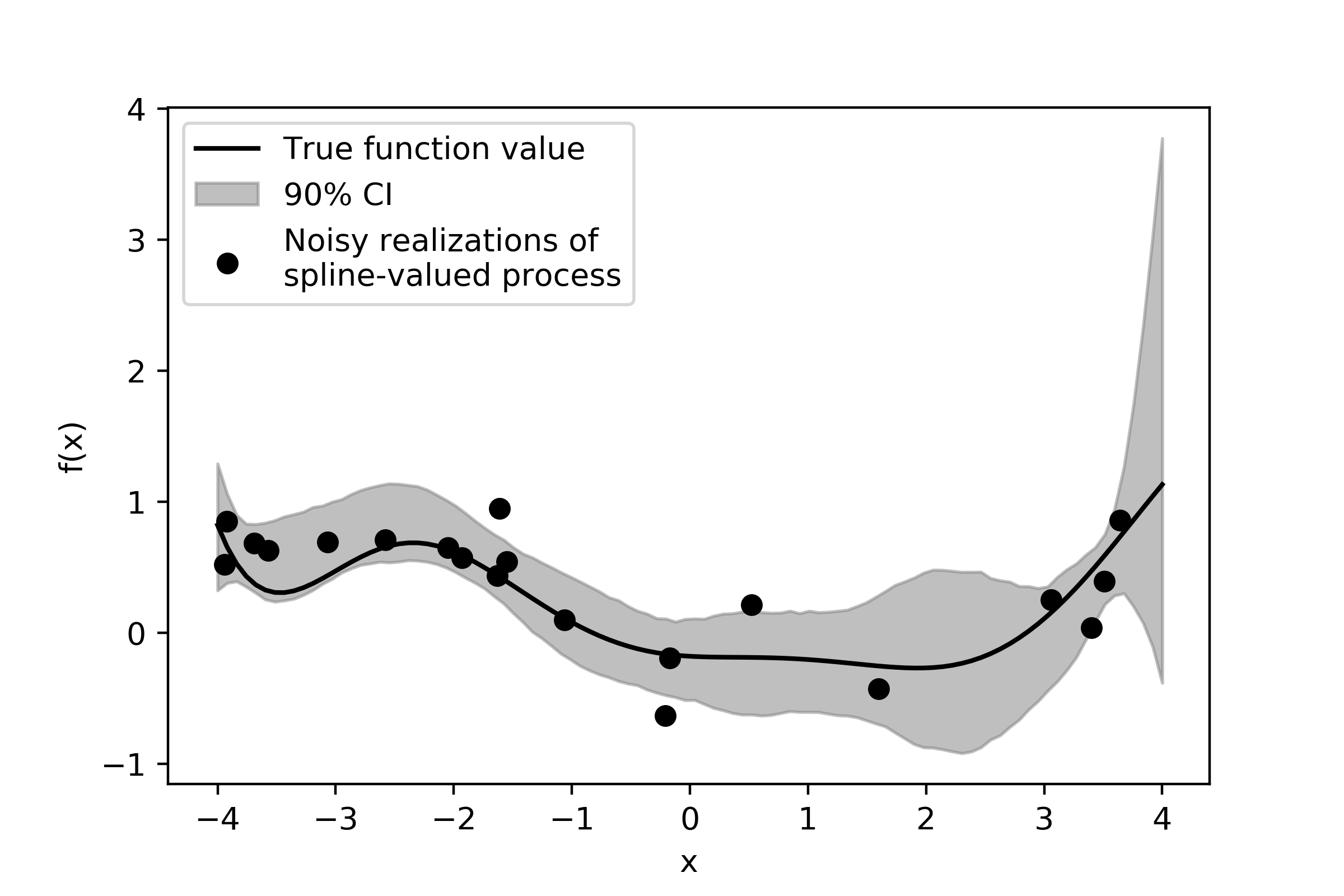
The strongest features of this curve are well-captured and the posterior estimate does cover the true spline curve value most of the time. We can see some edge effects here - as \(x\) gets larger and larger, the curve approaches the end of the domain and there are no more observed data points after \(x=4\). Thus, there is no data to constrain what the curve might look like in that region and consequently our uncertainty regarding what this function looks like is quite high.