Hamiltonian Monte Carlo for Hydrology, Part I

In a previous post I sketched out how to make a statistical model out of a simple ordinary differential equation. This is the first in a series of posts following my attempts to make a Bayesian version of a very simple conceptual hydrology model which is fit into a modern deep learning / Markov Chain Monte Carlo (MCMC) framework.

Why MCMC?

One of the scariest words that a hydrology modeler can hear nowadays is “equifinality”. In short, this is simply the situation where multiple different settings of the knobs and dials on a complicated hydrology simulation can lead to equally good accuracy in a testing phase. I’m not sure why this term had to be applied because this is a fundamental issue taught to every student of graduate statistics; in that discipline it is known as identifiability. Simply put, we want models in which we can uniquely identify the parameters. Unfortunately, highly parameterized hydrology models have faced major identifiability issues, prompting some in the earth sciences community to call attention to this crisis.

Bayesian methods in the statistical sciences are a natural way to tackle issues of identifiability because in that framework, we can use informative priors to shape the probability space of our model in such a way that makes a unique parameter solution much more likely to pop out. This touches on the topic of regularization in statistical learning theory. We regularize (i.e. push some model parameters to be either zero or non-impactful) when we have too many parameters for the model to be identifiable. This sort of logic is behind many of the greatest advances in machine learning as well. For those of you familiar with training of wide, deep neural networks, one way to substantially enhance the training process was to occasionally let some nodes in the network be blacked out and not interact with the rest of the network. Later on, it was discovered that this was, in fact, a form of Bayesian regularization even if the methods and model were not familiar to most conventional statisticians.

I want to fix the identifiability crisis in modern hydrology models by putting them in a Bayesian statistical framework. However, this poses a secondary issue: these models are complicated and often have latent processes within them that lead to enormous numbers of highly correlated parameters that cannot be tacked with the Metropolis algorithm. Metropolis and the Metropolis-Hastings algorithm are used extensively in hydrological applications of Bayesian statistics. There has been a cottage industry spawning a number of follow-on attempts to devise more accurate search heuristics within the hydrology community, though most of these lack any strong connection to the broader statistics literature. Most of us think of statistics as a nebulous gray cloud that occasionally drizzles significant p-values but virtually any situation in which predictive accuracy is desirable calls for some statistical know-how.

Hamiltonian MCMC

The most substantial development in applied Bayesian methods from the last decade is undoubtedly the development of Hamiltonian Monte Carlo (HMC) and subsequent refinements such as the No-U-Turn sampler as implemented in Stan and PyMC3. Put simply, HMC approaches use the curvature of the likelihood function in parameter space to determine where the MCMC sampler should move. This curvature is only defined for continuous likelihood functions (though we can typically use another algorithm for parameters that are discrete) and leads to highly efficient sampling for a wide class of problems. Specifically, HMC is very, very useful for sampling from posteriors over model parameter distributions in which the parameters are highly correlated. This is often the case in time series models. Hydrology models also appear to have this issue because there are frequently latent processes involved that can easily be simulated forwards but which are very difficult to estimate from observations in an inverse problem.

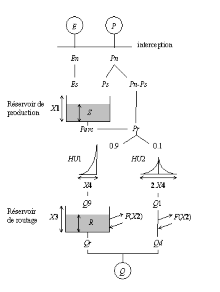
For an example of these latent processes, see the diagram for the conceptual hydrology model GR4J which I have stolen from the website of the Catchment Hydrology Research Group at IRSTEA in France. We typically have observations of the evaporation and precipitation as well as the discharge, but the amount of water in the two model reservoirs is unknown. Furthermore, since these reservoirs are filled and emptied according to difference equations, the reservoir level from day to day is going to have extremely high autocorrelations. This is why I want to use HMC to estimate the model parameters. Here, I am also describing the reservoir storage as a parameter even if it is not a parameter in the hydrologist’s sense of the word.

In part II of this series, I’ll include code for implementing a few subcomponents of GR4J in Theano, a powerful computational framework.