
Hamiltonian Monte Carlo for Hydrology, Part III
Published:
This is the third in a series of posts I am writing about my work on statistical hydrology. In posts I and II, I laid out the rationale for implementing a conceptual hydrology model in Theano and PyMC3. Here, I complete the implementation of GR4–a simple four parameter hydrology model–in PyMC3 and show that it can recover parameter estimates exactly with simulated data. To recap, I am doing this for multiple reasons. First, it allows for really, really fast Metropolis-Hastings updates because Theano is compiling all of this down to machine code for each sample execution. Second, it allows us to apply Hamiltonian Monte Carlo in case there are either lots of parameters or some of the parameters are highly correlated. Finally, a nice byproduct of this model is the fact that we can calibrate GR4J using backpropagation, just like in neural networks. For a simple watershed, we might not want to do this but if we have a model involving dozens of reaches and hundreds of parameters, it might be more effective than existing methods. All of this is possible because I have put GR4J in a framework that allows for automatic differentiation and thus the gradient of the model likelihood with regard to its parameters is available. This is a big, big advantage over gradient-free methods like genetic algorithms or similar approaches since we are always guaranteed to find at least a local minimum of our loss function. I won’t cover backpropagation-style calibration here but will give examples of applying Metropolis-Hastings and Hamiltonian Monte Carlo to the problem of estimating the parameters from synthetic streamflow data.
As in the previous post, I have written code to set up a PyMC3 distribution that is structured to copy the streamflow generation mechanistic model as explained in this article. For a summary of the model’s governing equations, you can also check out this link but it appears to occasionally be unreachable. My previous post includes a diagram that shows how the model is designed. The next few code cells describe the model logic in a way that can be parsed by Theano and PyMC3.
Runoff generation
The functions below are taken virtually unchanged from the second post in this series. In plain english, these functions represent the following process:
- Rainfall reaches the surface and some of it is evaporated right away. If the net evaporation is sufficiently low, some water will pass onto step 2.
- Some of this rainfall reaches the production reservoir - think of this as subsurface storage in the upper layers of soil or perhaps a shallow aquifer.
- The production reservoir loses some water due to evapotranpiration. Think of trees drawing water out of the vadose zone with their roots.
- As the production reservoir is leaky, some water will exit the reservoir and be generated as runoff. This runoff is used to calculate the total streamflow in later functions.
Step 2 is handled by calculate_precip_store, step 3 is handled by calculate_evap_store and step 4 is handled by calculate_perc. The logic for step 1 did not get its own function and is in the first few lines of streamflow_step.
import theano.tensor as tt
# Determines how much precipitation reaches the production store
def calculate_precip_store(S,precip_net,x1):
    n = x1*(1 - (S / x1)**2) * tt.tanh(precip_net/x1)
    d = 1 + (S / x1) * tt.tanh(precip_net / x1)
    return n/d

# Determines the evaporation loss from the production store
def calculate_evap_store(S,evap_net,x1):
    n = S * (2 - S / x1) * tt.tanh(evap_net/x1)
    d = 1 + (1- S/x1) * tt.tanh(evap_net / x1)
    return n/d

# Determines how much water percolates out of the production store to streamflow
def calculate_perc(current_store,x1):
    return current_store * (1- (1+(4.0/9.0 * current_store / x1)**4)**-0.25)
When called in sequence, these functions take in sequences of precipitation and evaporation data and calculate estimates of the amount of water exiting the catchment into the stream channel. The following code then takes this runoff and determines how long it takes for it to travel downstream. One nice thing about Theano is that these functions can be parsed and interpreted into a computational graph easily even though they look like nearly pure Python. In fact, if you just replaced the library theano.tensor aka tt with Numpy, then that code would work fine.
Streamflow routing and hydrograph generation
Next up comes the streamflow routing. The return values UH1 and UH2 partition a unit of runoff into today’s streamflow, tomorrow’s streamflow and so on. The parameter x4 controls how long it takes runoff to generate streamflow. There is a subtle point that must be addressed regarding this code, however. I make ample use of switch and maximum functions below which might appear to pose problems with regard to differentiability. However, since they are continuous and differentiable almost everywhere, Theano can get their gradients. I won’t go into detail here about why the model logic is structured this way; I recommend reading any of the online documentation for GR4J.
def hydrograms(x4_limit,x4):
    timesteps = tt.arange(2*x4_limit)

    SH1  = tt.switch(timesteps <= x4,(timesteps/x4)**2.5,1.0)
    SH2A = tt.switch(timesteps <= x4, 0.5 * (timesteps/x4)**2.5,0)
    SH2B = tt.switch(( x4 < timesteps) & (timesteps <= 2*x4),
                     1 - 0.5 * (2 - timesteps/x4)**2.5,0)

    # The next step requires taking a fractional power and
    # an error will be thrown if SH2B_term is negative.
    # Thus, we use only the positive part of it.
    SH2B_term = tt.maximum((2 - timesteps/x4),0)
    SH2B = tt.switch(( x4 < timesteps) & (timesteps <= 2*x4),
                     1 - 0.5 * SH2B_term**2.5,0)
    SH2C = tt.switch( 2*x4 < timesteps,1,0)

    SH2 = SH2A + SH2B + SH2C
    UH1 = SH1[1::] - SH1[0:-1]
    UH2 = SH2[1::] - SH2[0:-1]
    return UH1,UH2
Tying it all together
I used the functions declared in the previous code cells to handle some of the model logic but a large chunk of it still remains. My next function is going to be called for every timestep and calculates the various model quantities of interest.
def streamflow_step(P,E,S,runoff_history,R,x1,x2,x3,x4,UH1,UH2):

    # Calculate net precipitation and evapotranspiration
    precip_difference = P-E
    precip_net    = tt.maximum(precip_difference,0)
    evap_net      =  tt.maximum(-precip_difference,0)

    # Calculate the fraction of net precipitation that is stored
    precip_store = calculate_precip_store(S,precip_net,x1)

    # Calculate the amount of evaporation from storage
    evap_store   = calculate_evap_store(S,evap_net,x1)

    # Update the storage by adding effective precipitation and
    # removing evaporation
    S = S - evap_store + precip_store

    # Update the storage again to reflect percolation out of the store
    perc = calculate_perc(S,x1)
    S = S  - perc

    # The precip. for routing is the sum of the rainfall which
    # did not make it to storage and the percolation from the store
    current_runoff = perc + ( precip_net - precip_store)

    # runoff_history keeps track of the recent runoff values in a vector
    # that is shifted by 1 element each timestep.
    runoff_history = tt.roll(runoff_history,1)
    runoff_history = tt.set_subtensor(runoff_history[0],current_runoff)

    Q9 = 0.9* tt.dot(runoff_history,UH1)
    Q1 = 0.1* tt.dot(runoff_history,UH2)

    F = x2*(R/x3)**3.5
    R = tt.maximum(0,R+Q9+F)

    Qr = R * (1-(1+(R/x3)**4)**-0.25)
    R = R-Qr

    Qd = tt.maximum(0,Q1+F)
    Q = Qr+Qd

    # The order of the returned values is important because it must correspond
    # up with the order of the kwarg list argument 'outputs_info' to theano.scan.
    return Q,S,precip_store,evap_store,perc,runoff_history,R,F,Q9,Q1
I’ve made this function return a lot of arguments while only R, S and Q really need to be outputs. I did this because this section required significant debugging and I needed to see the results of all intermediate computations.
Next, I declare a bunch of Theano variables and feed them into my functions to make a valid computation graph.
import theano
theano.config.compute_test_value = "ignore"

precipitation = tt.vector()
evaporation   = tt.vector()

x1 = tt.scalar()
x2 = tt.scalar()
x3 = tt.scalar()
x4 = tt.scalar()
x4_limit = tt.scalar()

S0  = tt.scalar()
R0  = tt.scalar()
Pr0 = tt.vector()
This section does not actually compute any streamflow values - it simply compiles my Theano functions into a callable Python function that is very fast.
UH1,UH2 = hydrograms(x4_limit,x4)

outputs,out_dict = theano.scan(fn = streamflow_step,
                              sequences = [precipitation,evaporation],
                              outputs_info = [None,S0,None,None,None,
                                              Pr0,R0,None,None,None],
                              non_sequences = [x1,x2,x3,x4,UH1,UH2])

simulate = theano.function(inputs = [precipitation,evaporation,
                                     S0,Pr0,R0,
                                     x1,x2,x3,x4,x4_limit],
                           outputs = outputs)
Comparing streamflow outputs against a previous simulation
I have an existing non-Theano version of GR4J which I can compare my Theano code against. Below, I generate streamflow simulations using the same forcings as the other model and compute/plot differences between the two.
import pandas as pd
data = pd.read_csv('data_gr4j.csv')

test_x1       = 320.11
test_x2       = 2.42
test_x3       = 69.63
test_x4       = 1.39
test_x4_limit = 5
test_S0       = 0.6 * test_x1
test_R0       = 0.7 * test_x3

theano_simulated = simulate(data['P'].values,data['ET'].values,
                            test_S0,np.zeros(2*test_x4_limit-1),test_R0,
                            test_x1,test_x2,test_x3,test_x4,test_x4_limit)

theano_discharge = theano_simulated[0] # Picks out the simulated discharge

data = pd.read_csv('data_gr4j.csv')
plt.plot(theano_discharge-data['modeled_Q'],label='Difference between models')
_ = plt.xlabel('Timestep'), plt.ylabel('$$\Delta Q$$')
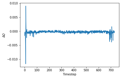
The discrepancy between the original model and this one is at most 1% and is usually much, much less. It looks the two are nearly identical in function and so the Theano-ized version is valid.
Running MCMC with GR4J in Theano / PyMC3
I went through all this work redoing a simple hydrology model so that I could fit it into PyMC3 and get either 1) tons of samples really, really quickly for Metropolis-Hastings, or 2) draw samples which are informed by the gradient of the model likelihood with Hamiltonian Monte Carlo. The PyMC3 distribution I’ve written out is useful for either case.
import pymc3 as pm
from pymc3.distributions import Continuous

class GR4J(Continuous):
    def __init__(self,x1,x2,x3,x4,x4_limit,S0,R0,Pr0,sd,precipitation,evaporation,truncate,
                *args,**kwargs):
        super(GR4J,self).__init__(*args,**kwargs)

        self.x1 = tt.as_tensor_variable(x1)
        self.x2 = tt.as_tensor_variable(x2)
        self.x3 = tt.as_tensor_variable(x3)
        self.x4 = tt.as_tensor_variable(x4)
        self.x4_limit   = tt.as_tensor_variable(x4_limit)

        self.S0 = tt.as_tensor_variable(S0)
        self.R0 = tt.as_tensor_variable(R0)
        self.Pr0 = tt.as_tensor_variable(np.zeros(2*x4_limit-1))
        self.sd = tt.as_tensor_variable(sd)

        self.precipitation = tt.as_tensor_variable(precipitation)
        self.evaporation   = tt.as_tensor_variable(evaporation)

        # If we want the autodiff to stop calculating the gradient after
        # some number of chain rule applications, we pass an integer besides
        # -1 here.
        self.truncate   = truncate

    def get_streamflow(self,precipitation,evaporation,
                      S0,Pr0,R0,x1,x2,x3,x4,x4_limit):

        UH1,UH2 = hydrograms(x4_limit,x4)
        results,out_dict = theano.scan(fn = streamflow_step,
                              sequences = [precipitation,evaporation],
                              outputs_info = [None,S0,None,None,None,
                                              Pr0,R0,None,None,None,None],
                              non_sequences = [x1,x2,x3,x4,UH1,UH2])
        streamflow = results[0]
        return streamflow

    def logp(self,observed):
        simulated = self.get_streamflow(self.precipitation,self.evaporation,
                                       self.S0,self.Pr0,self.R0,
                                       self.x1,self.x2,self.x3,self.x4,self.x4_limit)
        sd = self.sd

        return tt.sum(pm.Normal.dist(mu = simulated,sd = sd).logp(observed))
This is a lot to take in, but it’s mostly boilerplate. All I’ve really done with this class is tell PyMC3 to simulate streamflow given some parameters and inputs by iteratively calling streamflow_step within theano.scan. Then, it evaluates the likelihood function to penalize streamflow values which are far away from the observed data.
Metropolis results
With mostly uninformative prior distributions, the correct values of the parameters are easily computed using the Metropolis sampler as shown below. Note that the “observations” are actually synthetic outputs from the same hydrology model. The true parameters for that model run were declared in a previous code cell.
with pm.Model() as model:

    x1 = pm.Uniform('x1',lower = 100, upper = 1000)
    x2 = pm.Uniform('x2',lower = 1, upper = 10)
    x3 = pm.Uniform('x3',lower = 10, upper = 100)
    x4 = pm.Uniform('x4',lower = 1, upper = 5)

    x4_limit = 2*5-1
    S0 = pm.Uniform('S0',lower = 100, upper = 1000)
    R0 = pm.Uniform('R0',lower = 10, upper = 100)
    Pr0 = np.zeros(x4_limit)
    sd = 0.1

    streamflow = GR4J('streamflow',x1=x1,x2=x2,x3=x3,x4=x4,x4_limit=x4_limit,
                      S0=S0,R0=R0,Pr0=Pr0,sd=sd,
                      precipitation = data['P'].values,
                      evaporation = data['ET'].values,truncate=-1,observed = data['modeled_Q'])
    trace = pm.sample(step = pm.Metropolis(),draws = 10000)
100%|██████████| 10500/10500 [18:33<00:00, 9.38it/s]
While 10 iterations/second might not seem very impressive, it is important to remember that each of those is a simulation of streamflow across two years at a daily timestep and involves multiple vector operations. Also, I have specified the standard deviation for the normal log-likelihood function of the GR4J distribution manually. It would probably make sense to put some sort of prior distribution over the positive reals that penalizes long tails and prefers small variance.
As we can see from the posterior summaries below, the original parameter values are recovered with tight credible intervals.
pm.summary(trace)
x1:

  Mean             SD               MC Error         95% HPD interval
  -------------------------------------------------------------------

  326.755          18.635           1.859            [314.784, 365.150]

  Posterior quantiles:
  2.5            25             50             75             97.5
  |--------------|==============|==============|--------------|

  315.226        317.179        319.935        325.462        376.543


x2:

  Mean             SD               MC Error         95% HPD interval
  -------------------------------------------------------------------

  2.415            0.031            0.003            [2.363, 2.461]

  Posterior quantiles:
  2.5            25             50             75             97.5
  |--------------|==============|==============|--------------|

  2.331          2.406          2.421          2.435          2.457


x3:

  Mean             SD               MC Error         95% HPD interval
  -------------------------------------------------------------------

  68.671           3.049            0.303            [62.226, 71.320]

  Posterior quantiles:
  2.5            25             50             75             97.5
  |--------------|==============|==============|--------------|

  58.655         68.189         69.917         70.255         70.910


x4:

  Mean             SD               MC Error         95% HPD interval
  -------------------------------------------------------------------

  1.394            0.015            0.001            [1.376, 1.422]

  Posterior quantiles:
  2.5            25             50             75             97.5
  |--------------|==============|==============|--------------|

  1.379          1.386          1.389          1.396          1.439


S0:

  Mean             SD               MC Error         95% HPD interval
  -------------------------------------------------------------------

  196.485          12.115           1.208            [188.809, 222.487]

  Posterior quantiles:
  2.5            25             50             75             97.5
  |--------------|==============|==============|--------------|

  188.827        190.197        192.309        195.908        228.072


R0:

  Mean             SD               MC Error         95% HPD interval
  -------------------------------------------------------------------

  48.105           1.942            0.193            [43.852, 49.672]

  Posterior quantiles:
  2.5            25             50             75             97.5
  |--------------|==============|==============|--------------|

  41.658         47.937         48.891         49.109         49.614
Model fitting with HMC
As the next few cells show, model fitting also works with Hamiltonian MC. It is much, much slower per iteration (because of all the gradient calculations) but the samples will typically be drawn much more efficiently in terms of effective sampler size. Despite drawing an order of magnitude fewer samples than in the previous case with Metropolis-Hastings, the posterior summary variance is much smaller using HMC.
with pm.Model() as model:

    x1 = pm.Uniform('x1',lower = 100, upper = 1000)
    x2 = pm.Uniform('x2',lower = 1, upper = 10)
    x3 = pm.Uniform('x3',lower = 10, upper = 100)
    x4 = pm.Uniform('x4',lower = 1, upper = 5)

    x4_limit = 2*5-1
    S0 = pm.Uniform('S0',lower = 100, upper = 1000)
    R0 = pm.Uniform('R0',lower = 10, upper = 100)
    Pr0 = np.zeros(x4_limit)
    sd = 0.1

    streamflow = GR4J('streamflow',x1=x1,x2=x2,x3=x3,x4=x4,x4_limit=x4_limit,
                      S0=S0,R0=R0,Pr0=Pr0,sd=sd,
                      precipitation = data['P'].values,
                      evaporation = data['ET'].values,truncate=-1,observed = data['modeled_Q'])
    trace = pm.sample(draws = 1000)
100%|██████████| 1500/1500 [30:05<00:00, 1.54it/s]
pm.summary(trace)
x1:

  Mean             SD               MC Error         95% HPD interval
  -------------------------------------------------------------------

  320.271          2.125            0.105            [316.167, 324.471]

  Posterior quantiles:
  2.5            25             50             75             97.5
  |--------------|==============|==============|--------------|

  315.844        318.766        320.391        321.737        324.274


x2:

  Mean             SD               MC Error         95% HPD interval
  -------------------------------------------------------------------

  2.420            0.016            0.001            [2.391, 2.454]

  Posterior quantiles:
  2.5            25             50             75             97.5
  |--------------|==============|==============|--------------|

  2.389          2.409          2.420          2.431          2.453


x3:

  Mean             SD               MC Error         95% HPD interval
  -------------------------------------------------------------------

  69.587           0.667            0.033            [68.348, 70.943]

  Posterior quantiles:
  2.5            25             50             75             97.5
  |--------------|==============|==============|--------------|

  68.348         69.128         69.587         70.009         70.943


x4:

  Mean             SD               MC Error         95% HPD interval
  -------------------------------------------------------------------

  1.389            0.005            0.000            [1.379, 1.400]

  Posterior quantiles:
  2.5            25             50             75             97.5
  |--------------|==============|==============|--------------|

  1.379          1.386          1.389          1.393          1.400


S0:

  Mean             SD               MC Error         95% HPD interval
  -------------------------------------------------------------------

  192.184          1.467            0.070            [189.270, 195.063]

  Posterior quantiles:
  2.5            25             50             75             97.5
  |--------------|==============|==============|--------------|

  189.285        191.211        192.224        193.143        195.134


R0:

  Mean             SD               MC Error         95% HPD interval
  -------------------------------------------------------------------

  48.710           0.420            0.021            [47.836, 49.508]

  Posterior quantiles:
  2.5            25             50             75             97.5
  |--------------|==============|==============|--------------|

  47.896         48.454         48.682         48.989         49.611
Case study: time-varying parameters
Up until now, I have showed that HMC and normal Metropolis-Hastings can both be done with the Theano/PyMC3 code I wrote earlier. I would like to now show off an application that requires using something more sophisticated than the usual Gibbs sampling or Metropolis Hastings. I am going to make a synthetic dataset where the value of the GR4J parameter \(x_1\) is varying over time. Then, I will show that it can be recovered during inference, even if the observed data doesn’t look that different from the case where \(x_1\) is static.
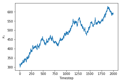
I’ve constructed a vector of \(x_1\) values by allowing it to follow a Gaussian random walk with a jump standard deviation of 3. As you can see, this let the value of \(x_1\) wander from 300 all the way up to 600.
T = 730
sd = 3
time_varying_x1 = 320.11 + np.cumsum(np.random.randn(730))* sd
_ = plt.plot(time_varying_x1),plt.xlabel('Timestep'),plt.ylabel('$$x_1$$')
The Theano code I wrote earlier can’t be reused for this example because now \(x_1\) is a sequence argument to theano.scan and I can’t think of a way to programatically control whether \(x_1\) is a scalar or vector. The next four code cells are nearly-identical repeats of my previous code blocks with the following alterations:
- The argument
x1tostreamflow_stepmust be passed as one of the first few arguments in the new version of this function,streamflow_step_tv_x1. x1is now one of thesequencesarguments totheano.scaninstead of one of thenon_sequencesarguments.
I could also change the other parameters to be time-varying but that would just complicate this test example.
def streamflow_step_tv_x1(P,E,x1,S,runoff_history,R,x2,x3,x4,UH1,UH2):

    # Calculate net precipitation and evapotranspiration
    precip_difference = P-E
    precip_net    = tt.maximum(precip_difference,0)
    evap_net      =  tt.maximum(-precip_difference,0)

    # Calculate the fraction of net precipitation that is stored
    precip_store = calculate_precip_store(S,precip_net,x1)

    # Calculate the amount of evaporation from storage
    evap_store   = calculate_evap_store(S,evap_net,x1)

    # Update the storage by adding effective precipitation and
    # removing evaporation
    S = S - evap_store + precip_store

    # Update the storage again to reflect percolation out of the store
    perc = calculate_perc(S,x1)
    S = S  - perc

    # The precip. for routing is the sum of the rainfall which
    # did not make it to storage and the percolation from the store
    current_runoff = perc + ( precip_net - precip_store)

    # runoff_history keeps track of the recent runoff values in a vector
    # that is shifted by 1 element each timestep.
    runoff_history = tt.roll(runoff_history,1)
    runoff_history = tt.set_subtensor(runoff_history[0],current_runoff)

    Q9 = 0.9* tt.dot(runoff_history,UH1)
    Q1 = 0.1* tt.dot(runoff_history,UH2)

    F = x2*(R/x3)**3.5
    R = tt.maximum(0,R+Q9+F)

    Qr = R * (1-(1+(R/x3)**4)**-0.25)
    R = R-Qr

    Qd = tt.maximum(0,Q1+F)
    Q = Qr+Qd

    # The order of the returned values is important because it must correspond
    # up with the order of the kwarg list argument 'outputs_info' to theano.scan.
    return Q,S,precip_store,evap_store,perc,runoff_history,R,F,Q9,Q1
class GR4J_tv_x1(Continuous):
    def __init__(self,x1,x2,x3,x4,x4_limit,S0,R0,Pr0,sd,precipitation,evaporation,truncate,
                *args,**kwargs):
        super(GR4J_tv_x1,self).__init__(*args,**kwargs)

        self.x1 = tt.as_tensor_variable(x1)
        self.x2 = tt.as_tensor_variable(x2)
        self.x3 = tt.as_tensor_variable(x3)
        self.x4 = tt.as_tensor_variable(x4)
        self.x4_limit   = tt.as_tensor_variable(x4_limit)

        self.S0 = tt.as_tensor_variable(S0)
        self.R0 = tt.as_tensor_variable(R0)
        self.Pr0 = tt.as_tensor_variable(np.zeros(2*x4_limit-1))
        self.sd = tt.as_tensor_variable(sd)

        self.precipitation = tt.as_tensor_variable(precipitation)
        self.evaporation   = tt.as_tensor_variable(evaporation)

        # If we want the autodiff to stop calculating the gradient after
        # some number of chain rule applications, we pass an integer besides
        # -1 here.
        self.truncate   = truncate

    def get_streamflow(self,precipitation,evaporation,
                      S0,Pr0,R0,x1,x2,x3,x4,x4_limit):

        UH1,UH2 = hydrograms(x4_limit,x4)
        results,out_dict = theano.scan(fn = streamflow_step_tv_x1,
                              sequences = [precipitation,evaporation,x1],
                              outputs_info = [None,S0,None,None,None,
                                              Pr0,R0,None,None,None],
                              non_sequences = [x2,x3,x4,UH1,UH2])
        streamflow = results[0]
        return streamflow

    def logp(self,observed):
        simulated = self.get_streamflow(self.precipitation,self.evaporation,
                                       self.S0,self.Pr0,self.R0,
                                       self.x1,self.x2,self.x3,self.x4,self.x4_limit)
        sd = self.sd

        return tt.sum(pm.Normal.dist(mu = simulated,sd = sd).logp(observed))
theano.config.compute_test_value = "ignore"
precipitation = tt.vector()
evaporation   = tt.vector()

x1 = tt.vector()
x2 = tt.scalar()
x3 = tt.scalar()
x4 = tt.scalar()
x4_limit = tt.scalar()

S0  = tt.scalar()
R0  = tt.scalar()
Pr0 = tt.vector()
UH1,UH2 = hydrograms(x4_limit,x4)

outputs,out_dict = theano.scan(fn = streamflow_step_tv_x1,
                              sequences = [precipitation,evaporation,x1],
                              outputs_info = [None,S0,None,None,None,
                                              Pr0,R0,None,None,None],
                              non_sequences = [x2,x3,x4,UH1,UH2])

simulate = theano.function(inputs = [precipitation,evaporation,x1,
                                     S0,Pr0,R0,
                                     x2,x3,x4,x4_limit],
                           outputs = outputs)
simulated_tv = simulate(data['P'].values,data['ET'].values,time_varying_x1,
                            test_S0,np.zeros(2*test_x4_limit-1),test_R0,
                            test_x2,test_x3,test_x4,test_x4_limit)

tv_discharge = simulated_tv[0] # Picks out the simulated discharge
Since \(x_1\) is time-varying and I have specified that it is allowed to change every timestep in my PyMC3 model which I’ll show later, there are 730 parameters to estimate and they are very highly correlated. This is a high dimension, high correlation problem which is exactly what HMC was designed for.
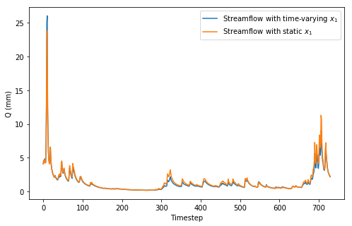
However, just because the parameter is allowed to vary over time does not necesarily mean that the observed streamflow is going to differ greatly from our previous case where \(x_1\) was assumed to be static. The streamflow plot below shows a comparison between the two cases and they are very, very similar.
plt.figure(figsize = (8,5))
plt.plot(tv_discharge,label='Streamflow with time-varying $$x_1$$'),
plt.plot(discharge,label='Streamflow with static $$x_1$$')
_ = plt.ylabel('Q (mm)'),plt.xlabel('Timestep'),plt.legend()
What’s interesting is that we can still get very good estimates on the value of \(x_1\) over time even though the observations don’t look very different. My PyMC3 code assumes that the standard deviation of the evolution of \(x_1\) is known (and this is rarely true in practice) but I’ll assume it is given. Placing a prior distribution on sd is a trivial extension of this model and does not complicate sampling much. The main difference between this and my previous PyMC3 model is that the parameter \(x_1\) is given an initial value from a uniform distribution but it is then allowed to wander over time with the GaussianRandomWalk distribution defined over 730 timesteps.
with pm.Model() as model:
    start_x1 = pm.Uniform('start_x1',lower = 100,upper = 1000)
    increment_x1 = pm.GaussianRandomWalk('increment_x1',sd=3,shape = 730)
    x1 = pm.Deterministic('x1',start_x1+increment_x1)
    x2 = pm.Uniform('x2',lower = 1, upper = 10)
    x3 = pm.Uniform('x3',lower = 10, upper = 100)
    x4 = pm.Uniform('x4',lower = 1, upper = 5)

    x4_limit = 2*5-1
    S0 = pm.Uniform('S0',lower = 100, upper = 1000)
    R0 = pm.Uniform('R0',lower = 10, upper = 100)
    Pr0 = np.zeros(x4_limit)
    sd = 0.1

    streamflow = GR4J_tv_x1('streamflow',x1=x1,x2=x2,x3=x3,x4=x4,x4_limit=x4_limit,
                      S0=S0,R0=R0,Pr0=Pr0,sd=sd,
                      precipitation = data['P'].values,
                      evaporation = data['ET'].values,truncate=-1,observed = tv_discharge)
    trace = pm.sample()
100%|██████████| 1000/1000 [9:47:28<00:00, 44.70s/it]/home/ubuntu/anaconda2/lib/python2.7/site-packages/pymc3/step_methods/hmc/nuts.py:459: UserWarning: Chain 0 reached the maximum tree depth. Increase max_treedepth, increase target_accept or reparameterize.
  'reparameterize.' % self._chain_id)
It’s important to notice that this took approximately 10 hours to draw 1000 samples, or roughly 2 samples per minute. This is quite slow but remember that this requires computing a 2000+ dimensional gradient through a computation graph with hundreds of layers (due to the temporal dependencies). This sampling was all done on a CPU; I would also like to try this on a GPU to see if any performance gains could be squeezed out.
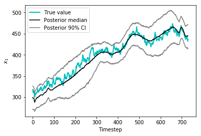
Fortunately, all that sampling was definitely worth it. The credible intervals below show that we’ve recovered relatively tight bounds on the value of \(x_1\) over time in the posterior disttribution.
mid   = np.percentile(trace['x1'],axis = 0, q = 50)
low   = np.percentile(trace['x1'],axis = 0, q = 5)
high  = np.percentile(trace['x1'],axis = 0, q = 95)

plt.plot(time_varying_x1[0:730],color='c',linewidth = 2, label = 'True value')
plt.plot(mid,color='k',label='Posterior median')
plt.plot(high,color='0.5',label='Posterior 90% CI')
plt.plot(low,color='0.5')
_ = plt.legend(),plt.xlabel('Timestep'),plt.ylabel('$$x_1$$')
This concludes my series of posts on model development in PyMC3. I may upload applications or extensions of this in the future. Feel free to contact me at ckrapu@gmail.com for any questions about how this works.