
Hamiltonian Monte Carlo for Hydrology, Part II
Published:
In this post, I’ll show how to implement part of a conceptual hydrology model in Theano and use it for sampling efficiently in PyMC3. The model I’ve chosen is GR4J and you can read about it at this website. It takes in four parameters and equal length time series of precipitation and evaporation and simulates streamflow. The model has two main components for generating runoff from rainfall and routing it via two hydrographs. I’ve grabbed a diagram from an existing paper and shown it below.
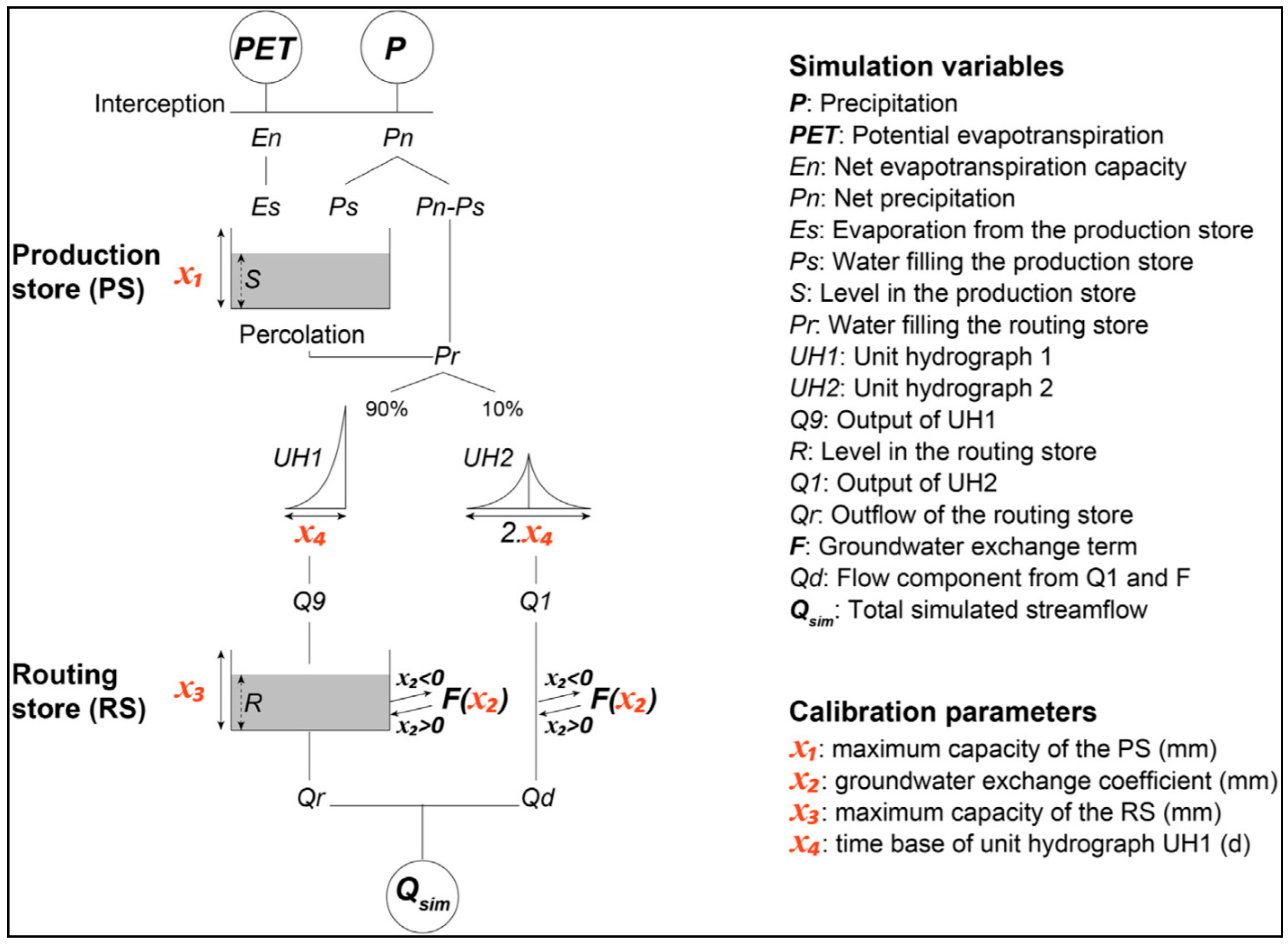
As you can see, streamflow is generated by computing the inflows and outflows from two storage reservoirs which have cross-timestep dependencies and which would thus frustrate any inference methods that can’t deal with correlated parameters. In the next section, I’ll set up the simulation and inference of the rainfall runoff half of GR4J.
Rainfall-runoff simulation
Here’s a function that generates time series of 1) water storage levels in the production reservoir, and 2) rainfall runoff which exits the production reservoir into the stream. All quantities are in millimeters and represent the average depth of the water over a river basin.
import numpy as np
def simulate_runoff(P,E,S0,x1):
    # Number of timesteps in simulation
    T    = len(P)
    S    = np.zeros(T)
    S[0] = S0
    Pr   = np.zeros(T)
    Perc = np.zeros(T)

    Ps = np.zeros(T)
    Es = np.zeros(T)
    Pn = np.maximum(P-E,0)
    En = np.maximum(E-P,0)

    for t in range(T):
        Ps[t] = x1 *(1.0 - (S[t]/x1)**2) * np.tanh(Pn[t]/x1) / (1 + S[t]/x1*np.tanh(Pn[t]/x1))
        Es[t] = S[t]*(2.0-S[t]/x1)*np.tanh(En[t]/x1)/(1+(1-S[t]/x1)*np.tanh(En[t]/x1))
        S[t]  = S[t]-Es[t]+Ps[t]
        Perc[t] = S[t]*(1-(1+(4.0/9.0*S[t]/x1)**4)**-0.25)
        if t+1 < T:
            S[t+1] = S[t] - Perc[t]
        Pr[t] = Perc[t] + Pn[t]-Ps[t]
    results = {'Pr':Pr,'S':S,'Ps':Ps,'Es':Es,'Pn':Pn,'En':En}
    return results
This model’s structure is pretty simple - it’s mostly straightforward arithmetic with a few tanh functions. Now that this is declared, I’m going to load some data and simulate the runoff.
import pandas as pd
import matplotlib.pyplot as plt
%matplotlib inline
forcings = pd.read_csv('forcing_gr4j.csv')
x1 = 320.11
numpy_simulated = simulate_runoff(forcings['P'].values,forcings['ET'].values,0.6*x1,x1)
numpy_simulated_runoff = numpy_simulated['Pr']
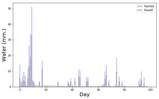
# Plot the precipitation inputs and resulting runoff
plt.figure(figsize = (10,6))
plt.bar(range(100),forcings['P'].values[0:100],color='b',label = 'Rainfall',alpha = 0.2)
plt.bar(range(100),numpy_simulated_runoff[0:100],color='k',label = 'Runoff',alpha = 0.2)
_ = plt.legend(),plt.ylabel('Water (mm.)',fontsize = 20),plt.xlabel('Day',fontsize = 20)
Recovering the original parameters
In order to use Theano, I need to first create some Theano-compatible functions for the GR4J model structure. Unfortunately, this means for-loops, Numpy and other Python essentials are unusable. The code below implements the model logic that I wrote out earlier in Numpy code, but does it in a way that Theano can use. The reason that all this has to be different is that Theano is not directly calculating the values that we want upon execution but is instead compiling a computational graph that will dramatically speed up the calculation of the simulated values in the future. Furthermore, Theano keeps track of the graph’s topology so that it can apply automatic differentiation for backpropagation or other gradient-based model fitting methods.
import theano.tensor as tt

# Determines how much precipitation reaches the production store
def calculate_precip_store(S,precip_net,x1):
    n = x1*(1 - (S / x1)**2) * tt.tanh(precip_net/x1)
    d = 1 + (S / x1) * tt.tanh(precip_net / x1)
    return n/d
#Ps[t] = x1 *(1.0 - (S[t]/x1)**2) * np.tanh(Pn[t]/x1) / (1 + S[t]/x1*np.tanh(Pn[t]/x1))
# Determines the evaporation loss from the production store
def calculate_evap_store(S,evap_net,x1):
    n = S * (2 - S / x1) * tt.tanh(evap_net/x1)
    d = 1 + (1- S/x1) * tt.tanh(evap_net / x1)
    return n/d

# Determines how much water percolates out of the production store to streamflow
def calculate_perc(current_store,x1):
    return current_store * (1- (1+(4.0/9.0 * current_store / x1)**4)**-0.25)

# Function to calculate contributions from each day, for each ordinate
# towards the hydrograph
def ordinates_step(current_precip,current_evap,current_store,x1):
    # Calculate net precipitation and evapotranspiration
    precip_difference = current_precip-current_evap
    precip_net    = tt.maximum(precip_difference,0)
    evap_net =  tt.maximum(-precip_difference,0)

    # Calculate the fraction of net precipitation that is stored
    precip_store = calculate_precip_store(current_store,precip_net,x1)

    # Calculate the amount of evaporation from storage
    evap_store   = calculate_evap_store(current_store,evap_net,x1)

    # Update the storage by adding effective precipitation and
    # removing evaporation
    store_updated = current_store - evap_store + precip_store

    # Update the storage again to reflect percolation out of the store
    perc = calculate_perc(store_updated,x1)
    store_updated = store_updated  - perc

    # The precip. for routing is the sum of the rainfall which
    # did not make it to storage and the percolation from the store
    current_rout = perc + ( precip_net - precip_store)
    return current_rout,store_updated,precip_store,evap_store,perc
To make sure that this matches our Numpy version, we’ll compile this as a function and see what results we get.
from theano.compile.nanguardmode import NanGuardMode
import theano
precipitation_tt = tt.vector()
evaporation_tt   = tt.vector()

x1_tt = tt.scalar()
S0_tt = tt.scalar()

outputs,out_dict = theano.scan(fn = ordinates_step,
                              sequences = [precipitation_tt,evaporation_tt],
                              outputs_info = [None,S0_tt,None,None,None],
                              non_sequences = [x1_tt])


simulate = theano.function(inputs = [precipitation_tt,evaporation_tt,S0_tt,x1_tt],outputs = outputs)
theano_simulated = simulate(forcings['P'].values,forcings['ET'].values,0.6*320.11,320.11)
theano_simulated_runoff = theano_simulated[0]
The next figure shows the distribution of per-timestep errors as measured by the difference between the two simulations divided by the Numpy simulation values over all 730 timesteps.
plt.figure(figsize = (8,5))
plt.hist((theano_simulated_runoff - numpy_simulated_runoff) / numpy_simulated_runoff,edgecolor='k',bins = 40)
_ = plt.ylabel('Counts'),plt.xlabel('% difference between Numpy, Theano')
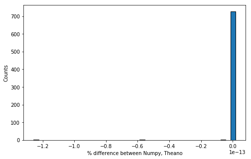
Again, all this plot shows is that the difference between the Numpy and Theano functions is essentially machine precision.
Next, I will wrap this up in a PyMC3 distribution which also includes Theano’s scan function to implement a for-loop in the Theano computational graph. This class functions within a larger PyMC3 model by taking in its inputs (which could also be random variables), simulating the runoff resulting from those inputs and making the likelihood function prefer input values which give a good match to the observed data.
import pymc3 as pm
import theano
from pymc3.distributions import Continuous
floatX = 'float64'

class GR4J_runoff(Continuous):
    def __init__(self,x1,S0,sd,precipitation,evaporation,truncate,
                *args,**kwargs):
        super(GR4J_runoff,self).__init__(*args,**kwargs)
        self.x1         = tt.as_tensor_variable(x1)
        self.S0         = tt.as_tensor_variable(S0)
        self.sd         = tt.as_tensor_variable(sd)

        # If we want the autodiff to stop calculating the gradient after
        # some number of chain rule applications, we pass an integer besides
        # -1 here.
        self.truncate   = truncate

        self.precipitation = tt.as_tensor_variable(precipitation)
        self.evaporation   = tt.as_tensor_variable(evaporation)

    def get_runoff(self,precipitation,evaporation,S0,x1):
        results,_ = theano.scan(fn = ordinates_step,
                              sequences = [tt.cast(precipitation,floatX),
                              tt.cast(evaporation,floatX)],
                              outputs_info = [None,S0,None,None,None],
                              non_sequences = x1,
                              truncate_gradient=self.truncate)
        return results[0]

    def logp(self,runoff):
        simulated = self.get_runoff(self.precipitation,self.evaporation,self.S0,self.x1)
        sd = self.sd

        return tt.sum(pm.Normal.dist(mu = simulated,sd = sd).logp(runoff))
The rest of my PyMC3 model is just going to be fairly standard stuff with some diffuse priors on the model parameters. We’ll first try Metropolis-Hastings on this model, since there are only two parameters.
T = 100                # This model will only be given 100 days' worth of synthetic runoff data to use for inference
with pm.Model() as model:

    sd = 0.1
    x1 = pm.Uniform('x1',lower = 100, upper = 1000)
    S0 = pm.Uniform('S0',lower = 100, upper = 1000)
    runoff = GR4J_runoff('runoff',x1,S0,sd,forcings['P'].values[0:T],forcings['ET'].values[0:T],
                         testval = theano_simulated_runoff[0:T],shape=T,
                         observed = theano_simulated_runoff[0:T])

    trace = pm.sample(live_plot=True,step=pm.Metropolis(),draws = 50000)
100%|██████████| 50500/50500 [04:46<00:00, 176.28it/s]
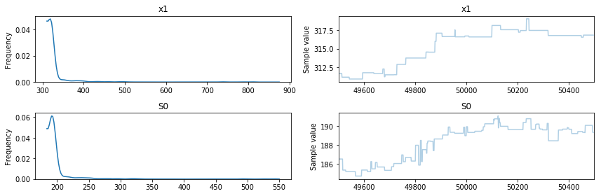
The live_plot keyword argument tells PyMC to spit out plots showing the variation of the draws as sampling proceeds as well as the density. This sampler is very fast at drawing samples and gives good credible intervals as we can see from the posterior summaries below. Recall that the true setting of x1 is 320.11 and the true setting of S0 was approximately 200.
pm.summary(trace,varnames = ['x1','S0'])
x1:

  Mean             SD               MC Error         95% HPD interval
  -------------------------------------------------------------------

  330.213          36.289           3.566            [310.944, 388.044]

  Posterior quantiles:
  2.5            25             50             75             97.5
  |--------------|==============|==============|--------------|

  311.884        318.050        321.494        325.286        436.058


S0:

  Mean             SD               MC Error         95% HPD interval
  -------------------------------------------------------------------

  199.649          26.913           2.648            [185.055, 244.054]

  Posterior quantiles:
  2.5            25             50             75             97.5
  |--------------|==============|==============|--------------|

  185.907        190.529        193.065        195.977        279.042
Next, I’ll try to solve the same problem with the No U Turn Sampler.
T = 730
truncate_gradient =   -1
with pm.Model() as model:

    sd = 0.1
    x1 = pm.Uniform('x1',lower = 100, upper = 1000)
    S0 = pm.Uniform('S0',lower = 100, upper = 1000)
    runoff = GR4J_runoff('runoff',x1,S0,sd,forcings['P'].values[0:T],forcings['ET'].values[0:T],
                        truncate = truncate_gradient,shape=T,
                         observed = theano_simulated_runoff[0:T])

    trace = pm.sample(draws = 500)
100%|██████████| 1000/1000 [03:32<00:00,  4.33it/s]/home/ubuntu/anaconda2/lib/python2.7/site-packages/pymc3/step_methods/hmc/nuts.py:451: UserWarning: The acceptance probability in chain 0 does not match the target. It is 0.923597808631, but should be close to 0.8. Try to increase the number of tuning steps.
  % (self._chain_id, mean_accept, target_accept))
pm.summary(trace,varnames = ['x1','S0'])
x1:

  Mean             SD               MC Error         95% HPD interval
  -------------------------------------------------------------------

  320.108          1.554            0.117            [317.211, 322.885]

  Posterior quantiles:
  2.5            25             50             75             97.5
  |--------------|==============|==============|--------------|

  317.211        319.123        319.993        321.161        322.885


S0:

  Mean             SD               MC Error         95% HPD interval
  -------------------------------------------------------------------

  192.059          1.257            0.094            [189.528, 194.136]

  Posterior quantiles:
  2.5            25             50             75             97.5
  |--------------|==============|==============|--------------|

  189.540        191.260        192.019        192.892        194.235
The posterior samples are similar to the ones calculated with the Metropolis sampler. Now that we can see that this approach can work with this hydrology model component, I’ll integrate this with a streamflow routing component in a future post so that the parameters of the entire GR4J model can be estimated with Theano and PyMC3.